
What This Article Argues
- Why most public explainers of MMM get the discipline structurally right but practically wrong.
- The judgement calls inside each stage that decide whether a model holds in front of your CFO.
- A test you can run on your own most recent MMM in under five minutes.
- How marketing mix modelling differs from multi-touch attribution and platform dashboards.
Marketing Mix Modelling has a credibility problem, and it is not the one most people think.
The problem is not that the discipline is too complex, too slow, or only for big brands. The discipline earned those reputations a decade ago, but they have not been true for some time. The problem is that most public explainers of MMM walk you through five stages as if they were a recipe. Gather the data. Apply some transformations. Run a regression. Validate. Decompose. Done. They make it sound mechanical, almost automated.
In reality, that is not what happens inside the work.
Specifically, inside every one of those five stages sits a judgement call. Ultimately, the judgement is what separates a model your CFO will sign off on from a model that collapses in the first five minutes of the debrief. After twenty years of building these models for global brands across retail, CPG, financial services, automotive, and direct-to-consumer, I have learnt that the mechanics are universal. The judgement is the work.
This article walks through the five stages and names the decision inside each one that determines whether the result is defensible. The figures referenced throughout are drawn from my forthcoming book with Dr. Firas Jabloun, What Great CMOs Need: An Executive Playbook for Modern Marketing Mix Modelling. Be the first to get it
A brief note before we start on MMM vs attribution. Marketing mix modelling is often discussed alongside multi-touch attribution (MTA) and platform attribution dashboards. They are not the same thing and they are not substitutes. MTA tracks individual user paths to conversion and answers questions about touchpoint ordering. Platform dashboards measure each channel inside its own walled garden, using the platform’s own definition of contribution. MMM measures all sales drivers simultaneously across the historical dataset, paid and unpaid, controllable and uncontrollable. The three methods sit in different parts of the measurement stack. The rest of this article is about MMM.
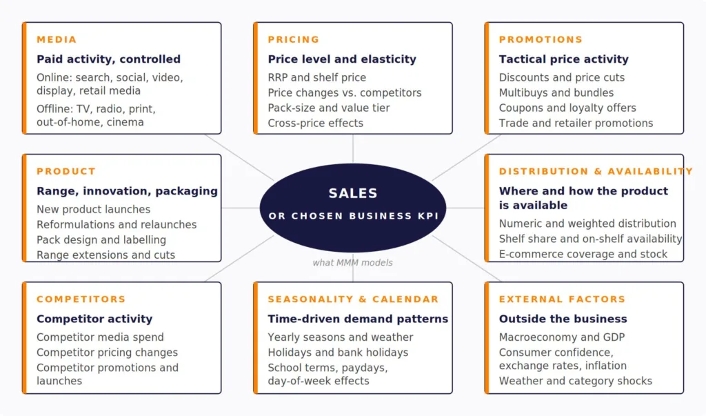
Figure 1. Factors influencing sales in an MMM context
Stage one: the data, and the gaps that quietly break the model
How does marketing mix modelling work in practice? It starts with data. The standard minimum is three years of weekly observations covering four input categories: KPI data (usually weekly revenue or sales volume); paid, owned, and earned media with spend and delivery metrics for every channel; marketing activities outside paid media, including pricing, promotions, and distribution; and external factors including seasonality, competitor activity, weather where relevant, and macroeconomic context. Figure 2 below lays out the full taxonomy of the four data categories and the typical owner of each. For a deeper treatment of the data required for MMM, see our dedicated guide.
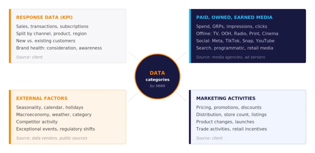
Figure 2. The four categories of data for Marketing Mix Modelling
What I have learnt to look for first is not what is in the dataset. It is what is missing.
A model that omits an important driver does not return a missing-driver warning. It silently transfers the missing driver’s effect to whichever variable in the model happens to be most correlated with it. When a brand runs a major distribution expansion that nobody mentions during the data exploration and scoping brief, the model attributes that growth to whichever media channel was active during the expansion window. The ROI of that channel inflates by a factor of two or three. The next budget round redirects spend towards what looks like the highest-returning channel, and the brand is now over-investing in a channel that was never doing the work.
A model that omits an important driver does not return a missing-driver warning. It silently transfers the missing driver’s effect to whichever variable in the model happens to be most correlated with it.
When a missing variable quietly distorts the results
I have seen this exact failure mode three times in the past five years. The most painful version involved a retailer who had quietly opened forty new stores during the modelling period. The brand team mentioned it on day one of the debrief, after the model had already been presented to finance. We rebuilt the model with the distribution variable correctly encoded. Television ROI fell by 38 per cent.
The judgement at this stage is not statistical. It is consultative. Consequently, the data scoping conversation has to be exhaustive, sceptical, and uncomfortable. Every plausible driver must be named, located, and decided on. Including it. Excluding it with a reason. Proxying it with the best available substitute. A model built on an incomplete brief is not wrong because of bad statistics. It is wrong because it answered a question nobody fully asked.
Stage two: transformations as commercial hypotheses, not parameter tuning
Once the data is assembled, the media variables in particular need transformation before they can enter the regression. Raw spend cannot model media response, because consumers do not respond to advertising the way a spreadsheet records it.
Specifically, two transformations carry most of the load. Adstock encodes the carryover effect of advertising over time. A consumer exposed to a television campaign in week one does not lose the impression by week two; it decays at a rate that differs by medium, creative, and audience. Diminishing returns encodes the saturation curve: each additional dollar in a channel generates progressively less incremental revenue. Both transformations are mathematical, but the parameter you set inside them is a commercial judgement.
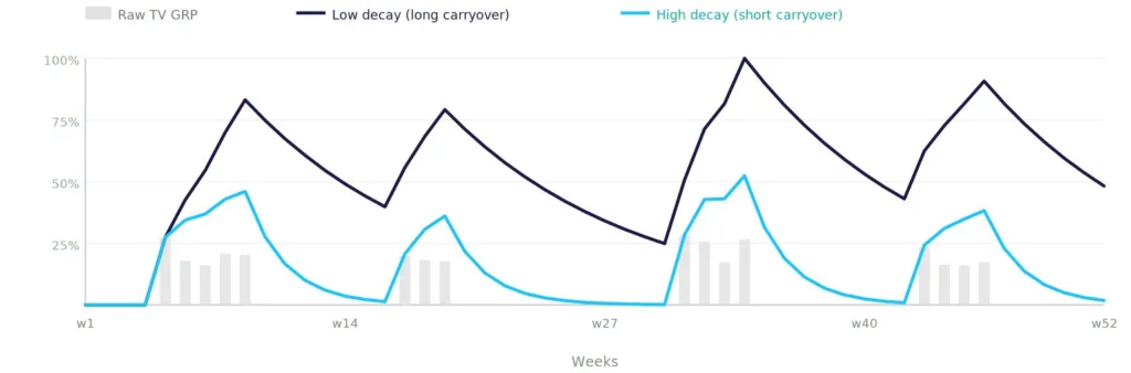
Figure 3. Adstock illustrated: raw TV GRP and two adstock transformations.
The mistake I see most often is treating the adstock decay rate as a free parameter for the model to optimise. Let the model search across a wide range of half-life values and it will always find one that fits the data better. The trouble is that the value the optimiser lands on may make no commercial sense. A 12-week half-life for a tactical promotion is mathematically a better fit than a one-week half-life, but no marketer in the room can defend the claim that a one-week promotion was still active in market three months later.
The honest way to set adstock is to ground it in evidence. Cross-correlation analysis on the raw dataset shows where the natural lag for each channel actually sits. Client knowledge about campaign structure and creative wear-out narrows the plausible range. In addition, the model then confirms or refutes inside that range. Anything else is curve fitting wearing methodological clothing.
Setting the diminishing returns curve shape
The Hill function for diminishing returns has the same property. The shape parameter determines whether the curve is C-shaped, meaning returns diminish from the first dollar, or S-shaped, meaning a threshold of spend is needed before response builds. These are two different commercial realities. An always-on channel reaching a mature audience is C-shaped. A brand-building campaign that needs to build awareness before purchase consideration registers is S-shaped. Choosing the curve shape is a planning decision, not a fitting one.
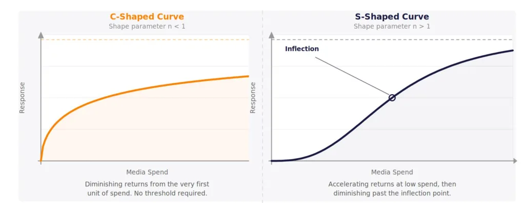
Figure 4. C-shaped and S-shaped diminishing returns curves (Hill function).
Every transformation parameter is a hypothesis about commercial reality. A hypothesis the model can confirm or refute, but not invent.
The judgement at this stage is to refuse to delegate it to the optimiser. The parameter range has to come from the marketing reality of the channel. The model lives inside that range.
Stage three: the regression, and what R-squared is actually telling you
With transformations applied, the regression estimates how much of the observed movement in the KPI is attributable to each variable. Ordinary least squares (OLS) is the foundational technique. Log-linear, pooled, nested, hierarchical, and Bayesian regression are the variants you apply when the data structure or the commercial question demands them. Open-source frameworks take different paths: Meta’s Robyn applies ridge regression as a Bayesian-style variant to handle multicollinearity, while Google’s Meridian uses a hierarchical Bayesian approach. Commercial platforms typically support several. The technique chosen is far less important than how it is specified and validated.
Specifically, R-squared is the metric most clients ask about first. It measures the proportion of variance in the KPI that the model accounts for. An R-squared of 0.88 means the model explains 88 per cent of the total variation in weekly sales across the modelling period. For a weekly national sales model, 0.85 is a reasonable minimum, and consistently above 0.90 is well-specified.
R-squared alone is not a guarantee of anything. It rises mechanically with every variable you add to the model, regardless of whether the new variable contributes genuine explanatory power. Adjusted R-squared corrects for this. If R-squared rises but adjusted R-squared declines as you add variables, the model overfits rather than improves.
Key fit metrics beyond R-squared
The other fit metric that matters in practice is MAPE, the mean absolute percentage error. It measures how accurately the model reproduces actual data, period by period. Below 10 per cent is excellent for stable categories. Between 10 and 15 per cent is acceptable for more volatile markets. Above 20 per cent signals a model that should not be used for forward planning. For a full treatment of the key statistical tests for marketing mix modelling, including R-squared, MAPE, and Durbin-Watson, see our dedicated article.
A model that fits the data but contradicts the market is not a measurement. It is an expensive distraction.
When statistical fit is not enough
But here is the move that most explainers miss. A model with R-squared of 0.92 and MAPE of 7 per cent can still be unusable. I have rejected models with those numbers. The reason is that a model can fit the past perfectly while still producing channel contributions that contradict everything the brand team knows about its market. The model with the best statistical fit is not the model that ships. The model that ships is the one that is both statistically sound and commercially coherent.
The judgement at this stage is to remember that statistical fit is necessary but not sufficient. The next stage is what closes the gap.
Stage four: the marketing mix modelling validation framework, in three stages
Validation is where most public explainers compress everything into a single line: you test the model against historical data to check accuracy. That is true and it is also not enough. A serious validation discipline has three sequential stages, and all three must pass.
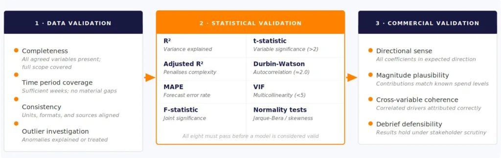
Figure 5. The three-stage validation framework
Data validation comes first. Completeness across all agreed variables. Time period coverage with no material gaps. Consistency in units, formats, and sources. Outliers investigated and either explained or treated. If the data is not clean at this stage, no amount of statistical sophistication downstream rescues it.
Statistical validation is the second stage. This is where the eight-diagnostic battery applies. R-squared above 0.85 for weekly national models. Adjusted R-squared rising as variables are added, not falling. MAPE below 10 per cent for stable categories, below 15 per cent for volatile ones. The F-statistic significant at the 5 per cent level for the variable set as a whole. The t-statistic above 2 in absolute value for each individual variable. Durbin-Watson between 1.5 and 2.5, ideally close to 2.0, to confirm no autocorrelation in the residuals. Variance inflation factor below 5 for each variable, to control multicollinearity. Jarque-Bera testing that residuals are not significantly non-normal. A model that passes seven of eight is not a valid model.
Commercial validation: the stage most easily skipped
Commercial validation is the third stage and the one most easily skipped. Directional sense: every coefficient moves in the expected direction. Magnitude plausibility: contributions match known spend levels and category benchmarks. Cross-variable coherence: correlated drivers are attributed correctly between themselves. Debrief defensibility: the results hold under stakeholder scrutiny without the modeller needing to explain anomalies away.
Validation is not a quality check tacked onto the end. It is a discipline that runs alongside the modelling from the first iteration
A case where a statistically sound model failed the debrief
The story I tell juniors is this one. A model I built four years ago passed every statistical diagnostic. R-squared of 0.91. MAPE of 8 per cent. Every t-statistic above 2. Durbin-Watson at 1.97. VIF clean across the board. The model attributed 31 per cent of incremental revenue to a digital display campaign that the brand had paused halfway through the analysis window.
The model was statistically beautiful and commercially nonsense. We went back, found the omitted variable that explained the spurious attribution, rebuilt, and the display contribution settled at 9 per cent. The first model would have passed any peer review of its statistics. It would have failed the debrief in front of the CFO.
The judgement at this stage is that validation is not a quality check tacked onto the end. It is a discipline that runs alongside the modelling from the first iteration, surfacing problems early enough to resolve them analytically rather than explain them away at the debrief.
Stage five: reading the results, and the move from output to decision
A validated model produces three classes of output. Contribution analysis decomposes the KPI into base sales, seasonality, promotions, each media channel, pricing, competition, and any other variable in the model. Return on investment by channel divides each channel’s contribution by its spend, producing the canonical efficiency reading every marketer recognises. Saturation curves plot the response-to-spend relationship for each channel, showing where it is under-invested, optimally invested, or in diminishing returns.
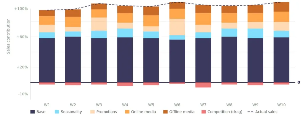
Figure 6. Sales decomposition contribution chart
However, the numbers on their own are not yet a decision. The move from output to decision is where the model earns its commercial value.
Budget optimisation is the most direct application. Given the saturation curves of each channel and a total budget envelope, the model identifies the allocation that maximises total revenue. In practice, the recommendation is rarely uniform. A channel sitting deep in saturation should lose spend, even if its absolute ROI is positive. A channel in the early-spend zone of its curve should gain spend, even if its current contribution is small. The instinct to redirect from the worst-performing channel to the best-performing one is often wrong. The right move is to redirect from the most-saturated channel to the least-saturated one, which is a different calculation.
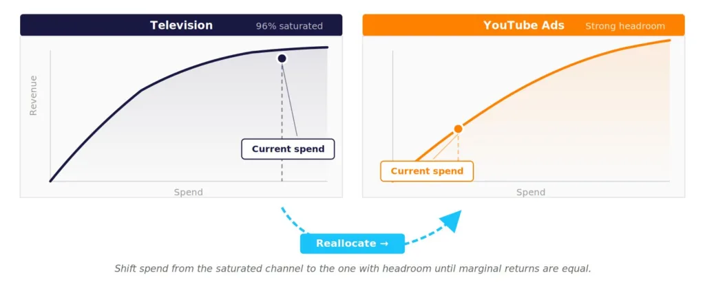
Figure 7. Budget reallocation between channels at different points on their diminishing returns
Scenario planning and the case for continuous measurement
Forecasting and scenario planning is the second application. With the model in place, you can simulate the revenue impact of changing the budget envelope, shifting allocation between channels, launching a new channel, or absorbing a planned price change. The accuracy of those scenarios depends on how confidently you can extrapolate the response curves into unobserved spend ranges. A model can tell you what happens at 10 per cent above current spend in a channel. It is more cautious at 50 per cent above, and silent beyond the data it has seen. Where experimentation data is available, MMM combined with experiments (Model Plus Experiments) extends the confidence range significantly.
I have learnt to push hard on the question of what the model is being asked to do next. The most valuable MMMs are the ones connected directly to the planning cycle that follows them. A model produced once a year, in a slide deck, by a consultancy, three months after the period it modelled, is producing reports. A model refreshed continuously, integrated into the brand’s planning workflow, producing decisions before the budget round closes, is producing value.
This is what MASS Analytics means by Always-ON MMM. The model is not a periodic study. It is the operating system for marketing measurement, refreshing as new data arrives, calibrated by experiments where available, and surfacing the next decision before the window to make it closes. For a broader view of what this looks like in practice, see the five pillars of a best-in-class MMM capability.
The model that ships is not the best model. It is the best model integrated into the planning cycle that follows it.
Designing for the decision, not the output
The judgement at this stage is to design for the decision, not for the output. A model with no consumer downstream is an expensive academic exercise.
Marketing mix modelling Frequently Asked Questions
Is marketing mix modelling the same as multi-touch attribution?
No — the two methods are fundamentally different and not substitutes for each other. MMM measures all sales drivers simultaneously across the historical dataset using aggregate weekly data. It captures offline channels, pricing, distribution, and competitive activity that MTA cannot see.
Multi-touch attribution, by contrast, tracks individual user paths to conversion using cookie or device-level data. It answers questions about touchpoint ordering within a single user journey, but it is blind to anything that happens outside a tracked digital session. How MMM compares with other measurement techniques is covered in depth in our broader guide. The two methods answer different questions and sit in different parts of the measurement stack.
What is the minimum data requirement for a marketing mix modelling project?
Specifically, three years of weekly observations is the standard minimum. This window covers two full annual cycles plus a year of variation, which is what the model needs to calibrate seasonal patterns and carryover effects reliably.
Two years is workable for stable categories with low seasonality, but it produces less confident saturation curves. Less than two years is rarely sufficient — the model simply does not have enough variation to separate the signal from the noise across channels and seasons.
How long does an MMM project take to build?
An initial build from clean data to validated model typically runs six to twelve weeks. The first half covers data assembly, quality assurance, and variable definition. The second half is modelling, validation, and the commercial debrief.
Always-ON implementations work differently. After the initial build, the model refreshes continuously as new data arrives, replacing the periodic-study cycle with an integrated measurement layer that updates in step with the business.
You made it to the end. If this raised more questions than it answered, that is exactly what What Great CMOs Need: An Executive Playbook for Modern Marketing Mix Modelling is built for. Be the first to get it!
What every marketing mix modelling project has in common, and what every project does differently
The MMM process is universal. The MMM methodology is universal. Every credible marketing mix modelling project, regardless of vendor or sector, moves through data, transformation, regression, validation, and reading the results. The five-stage spine is not a competitive differentiator. It is the cost of entry.
What differentiates one MMM from another is the judgement applied inside each stage. The completeness of the data brief. The discipline of grounding transformation parameters in commercial reality rather than statistical fit. The willingness to reject a statistically beautiful model on commercial grounds. The validation framework that requires all three stages to pass, not just the statistical one. The integration into the planning cycle that turns outputs into decisions.
Twenty years of building these models has taught me that the practitioners who get this right share a habit. They treat every parameter, variable, and validation as a hypothesis about commercial reality, not a free degree of freedom for the optimiser to consume. The model is in service of the business question. The business question is not in service of the model.
The model is in service of the business question. The business question is not in service of the model.
If you are running an MMM today and want to know whether yours is built this way, the test is simple. Pull the most recent debrief. Find a channel contribution that surprised you. Ask the modelling team to walk you through which judgement call inside which stage produced that number, and what evidence grounded the judgement.
If the answer is methodologically specific, you are working with the right team. If the answer is a statistical fit metric without the commercial reasoning behind it, you are looking at curve fitting in a presentation deck.
How much of your last budget round was built on a model whose judgement calls you could defend in front of your CFO?
Key Takeaways
- Marketing mix modelling is a five-stage statistical process: data, transformations, regression, validation, and reading the results.
- The model that ships is decided by judgement at each stage, not by the highest R-squared in the run.
- Validation has three sequential parts: data, statistical, commercial. All three must pass.
- Transformation parameters are commercial hypotheses grounded in evidence, not free degrees of freedom for the optimiser.
- MMM measures all sales drivers simultaneously across the historical dataset. MTA and platform dashboards do not.