Regression Analysis for Marketing Mix Modeling

This comprehensive guide will give you an overview of what regression analysis is, its different types and how you can leverage it in Marketing Mix Modeling.

Regression analysis is an important part of model building, the fourth phase in the MMM workflow. It is a powerful approach used to uncover and measure the relationship between a set of variables and a specified KPI. It also predicts future outcomes, which makes it a very useful and common technique in building marketing mix models.

Regression analysis has prescriptive power. In fact, analysts often use it to predict the value of a variable (the dependent variable, or the KPI of interest) based on other variables (the independent variables).

By the end of this blog, you will be well-versed in the basics of regression analysis. You’ll also be ready to start making data-driven decisions by interpreting the results of your regression analysis.

Let’s start first by defining a key component of regression analysis.

Why is Correlation Crucial for Regression Analysis?

Correlation – or Pearson’s Coefficient of Correlation – is a key statistic. You therefore need to compute and analyze it as part of the explore phase of the MMM workflow.

Pearson’s Correlation coefficient is a standardized covariance:

• Measures the relative strength of the linear relationship between two variables
• Unit-less
• Ranges between -1 and 1
• The closer to -1, the stronger the negative linear relationship
• The closer to 1, the stronger the positive linear relationship
• The closer to 0, the weaker any linear relationship

This metric is useful to appreciate the strength of the relationship between two variables. However, the presence of a correlation does not necessarily mean causality. Possible explanations include:

• Direct cause and effect: water causes plants to grow
• Both cause and effects: coffee consumption causes nervousness; nervous people have more coffee.
• Relationship caused by third variable: death due to drowning and soft drink consumption during summer. Both variables here are related to heat and humidity (third variable).
• Coincidental relationship: an increase in the number of people exercising and an increase in the number of people committing crimes.

Correlation is a key component you calculate and analyze as part of the MMM workflow. However, it is important to mention that it can only depict linear association and it fails to depict any non-linear associations.

The Simple Linear Regression

What is the impact of advertising on sales? Or in other terms, if you know how much budget you are investing in advertising, are you capable of forecasting how much sales you can achieve? Regression analysis allows you to do that.

But before dealing with real-life examples that require elaborate types of Regression, let’s start simple. So we’ll use the Simple Linear Regression to fully understand how the process works.

First, you need to collect a sample of data periods about $x$ — in this case, the advertising spend. You also need a sample of data periods about $y$ — in this case, the sales volume.

Then, you use the regression technique to estimate the relationship between the variations period on period of advertising and the variations in sales. Statistically speaking this means estimating the coefficients ${\beta }_0$ and ${\beta }_1$.

Once you estimate these, you can discover the level of sales you could achieve for a given advertising spend.

Now that we got the business element explained, let’s dive into the mathematical side of the simple linear regression:

The equation of a simple linear regression depicts a dependency relationship between two variables or two sets of variables. The first set is the dependent variable, and the second set holds the predictors, or independent/explanatory variables. Because this is “simple” linear regression, the independent variables set contains only one variable. So you use this variable to predict the outcome of the dependent variable.

To predict the outcome for different values (or scenarios of $x$) the analyst needs to estimate β₀ and β₁ from the data collected.

y = Dependent Variable.

x = Independent Variable.

β₀ = Intercept.

β₁ = Slope.

ε = Error term.

ε is a normal random variable with E(ε) = 0 and V(ε) = σ², i.e. ε ~ N(0, σ²)

---

Parameters

• β₀ and β₁ are unknown, and the goal is to estimate them using the data sample.
• β₀ is the base.
• β₁ represents the coefficient of the independent variable x.
• ε is the error term or residual. In regression analysis, it is important that the error term is random and is not influenced by any other factor. In particular, it should be as small and as random as possible.

How Does Linear Regression Work?

Let’s consider the following equation that models the impact of advertising on sales.

When data is plotted, we obtain the following chart where each point has an $x$ coordinate and $y$ coordinate:

• X represents the advertising budget.
• Y coordinates represent the sales achieved for a particular advertising spend (value of X).

The goal of the simple regression analysis is to find the line (i.e. the intercept and slope) that goes through the maximum data points in this chart. In doing so, this line minimizes the distance between each point and its projection on the “searched for” line.

The blue line is the best line and is the estimate or $\stackrel{}{}$. To do this, you obtain point estimates by projecting the initial data points (the dots) on the estimate line $\stackrel{}{}$.

The fitted line equation is: $\widehat{y}={\widehat{\beta }}_0+{\widehat{\beta }}_{1}x$
Note here that it is no longer about β₀ and β₁, but rather their hat variations, because you estimate the parameters β₀ and β₁ using ${\widehat{\beta }}_0$ and ${\widehat{\beta }}_1$, based on the sample of data collected.

The intercept is where the line crosses the y-axis, the value of sales when advertising spend is zero. In other words, that represents the base sales.

The slope is that of the curve of the fitted line. Specifically, two coordinates, $x$ and $y$, define any data point. Projecting a point onto the line gives its estimate $\widehat{y}$.

The orange dot marks the difference between the point’s initial position and its projection on the line — this difference is the error term. The smaller the error term, the better the regression line estimates the relationship between $x$ and $y$.

OLS: Ordinary Least Squares is the method used to estimate the parameters β₀ and β₁ and minimize the error term.

How Refined Could Your Forecast With Regression Analysis Be?

To estimate the sales volume for a given period, a simple method quotes the average sales of previous periods. In other words, it’s a forecasting method based on the average. If you use regression instead, the forecast becomes a little more sophisticated.

In regression analysis, we illustrate a simple idea. Once you know the advertising budget you plan to deploy, you can use that information about the “independent variable” to refine your sales forecast. A forecast based on regression should outperform one based on the simple average method.

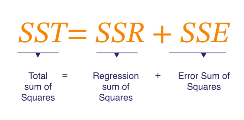
How much does regression improve predictions over the simple average method? This leads us to introduce the concept of variance decomposition. The aim is to achieve a decomposition of the total variance SST (sum of squared total) into two components:

1. SSR represents what the model — the regression line — explains.
2. The residual part (the unexplained part) of the equation, which is SSE: The Sum of Squared Error.

Total variation consists of two parts

In the following chart:

The projection of a specific point on the blue line represents the estimate $\widehat{y}$.

The difference between the estimate and the yellow line represents the gain from using regression, instead of the simple average method, for forecasting.

Meanwhile, the difference between the real point (the red point in the graph) and its projection on the yellow curve is the error, or the residual.

The ideal situation is one where the sum of squared error (the residual) is very small compared to the SSR. In other words, SSR is the sum of squared regression.

R-Squared (R²): How Much Variance Is Explained By The Model?

Those who are familiar with Regression or Marketing Mix Models have certainly heard about R² multiple times. But what does it really mean in Layman’s terms?

SSR represents what the model — the regression line — explains.

$R^2=\frac{\mathrm{SSR}}{\mathrm{SST}},\text{where:}0\le R^2\le 1$

R² simply represents the portion of the variance in the dependent variable that the model, or the independent variable, explains. The higher the R², the better. In our sales/advertising example, if R² equals 70%, movements in the advertising variable explain 70% of the variation in the sales data. So, advertising can explain 70% of the variation in the dependent variable (sales).

R² is a very important metric in Marketing Mix Models. Specifically, it indicates how successful the model, and its variables, are at explaining the variations in the modeled KPI.

How Accurate Is Your Model? The Standard Error of The Estimate

This is a measure of the accuracy of the model. It captures the typical size of the residuals, the differences between the real $y$ values and their estimates ŷ. In ordinary least squares the residuals average to roughly zero, so what matters is their spread, not their mean. This statistic is very useful as it shows how accurate the results of the modeling are and the prediction power of the model.

Tip: Analyze your residuals and plot them at all times! Make sure the OLS assumptions are respected and use the relevant statistics to establish your assessment (DW, VIF, Normality test, homoscedasticity etc.).

T-Stat: How Reliable is Your Model?

The t-stat is a standard output of the model and a very important statistic to look at when building MMM models. Remember that the dataset used to create a regression model is a sample. You use that sample to estimate the parameters β₀ and β₁ at the population level. It is therefore very important to ensure that the estimates we obtain from the sample are reliable. In particular, they need to be good estimates for the population parameters. In other terms, if we had picked up another sample from the same population, would we have obtained the same estimates (within a certain confidence interval)? That is exactly what the t-stat is for.

As a rule of thumb, the t-stat should be above 2 to make sure that we are reporting reliable impacts.

What Does Real-life Regression look like?

Now that you explored how Simple Linear Regression works, it’s time to move to what happens in real life when working on an MMM project.

There are many variations of Regression analysis that are used in Marketing Mix Modeling:

In this part of the article, we’re going to discuss the Multiple Linear Regression.

Multiple Regression

Multiple Regression is as simple as stating that the period-on-period movements/variations in the dependent variable (the KPI that we are interested in modeling, e.g. sales) are not any more explained by the variations of the movements of one single variable, but rather by the movement of multiple variables.

This is of course a more representative setting. Analysts rarely use simple linear regression in real-life MMM projects, since it is too simplistic to handle the complexity of consumer behavior and the media landscape.

Thus, when the analyst starts adding more variables into the regression equation, they move from simple regression setting to multiple regression setting.

In a typical marketing mix modeling project, multiple variables impact the sales performance, e.g.:

• Media investments (online and offline)
• Promotional Activity
• Seasonality
• Distribution
• External Factors

To be able to measure the impact of those variables on sales or any other chosen KPI, the analyst needs to build a robust model which accounts for all the variables influencing the movement of sales.

• ${\beta }_0,{\beta }_1,\cdots ,<mi>\; </mi>{\beta }_k$: are population model parameters (coefficients) to be estimated from the sample.
• ${\beta }_0$ represents the base, a very important concept in MMM.
• $x_1,x_2,\cdots ,<mi>\; </mi>x_k$ are the independent variables influencing sales.
• The term ${\beta }_k{x}_k$ represents the contribution of the variable $x_k$ on sales: i.e. how much sales are driven by the variable $x_k$ (incremental impact)
• $\epsilon$: are the error terms, assumed to be independent and following the normal distribution with 0 mean and constant variance.

Estimating this model will help the business better predict their sales performance. In that, they gain insights into:

• The impact of every media channel on sales be it online or offline.
• How much budget to allocate to media before reaching saturation.
• Which promotional mechanics to utilize.
• The distribution levels to maintain.
• How they could leverage seasonality.

Once you estimate the parameters ${\beta }_0,{\beta }_1,\cdots ,\text{and}{\beta }_k$, you can plug those values into any media and marketing scenario and predict the incremental sales you will make. As a result, this becomes a powerful tool for decision making.

How The Parameters Are Estimated

The process is the same as that of the simple linear regression. The goal is to minimize the residuals, which is the difference between $y$ and ŷ. The method of estimation is also the same: the Ordinary Least Squares (OLS) method. Specifically, it finds the estimates of ${\beta }_0,{\beta }_1,{\beta }_2,\dots ,$ and ${\beta }_4$ that minimize the sum of the squared error:

Coefficient Interpretation

In a given equation, the estimated coefficient $\widehat{{\beta }_k}$ related to the advertising variable $x_k$ would represent the sensitivity of the dependent variable to variations in the independent variable $x_k$.

In a given equation, the estimated coefficient $\stackrel{}{{\beta }_k}$ relates to the variable $x_k$. In other words, it represents the sensitivity of the dependent variable to variations in the independent variable $x_k$.

For instance, if $x_k$ represents the search activity expressed in terms of millions of impressions, then a 1 unit movement in $x_k$ (i.e. 1 million impressions) yields an estimated $\widehat{{\beta }_k}$ unit increase in sales. This holds while keeping all the other variables in the equation (seasonality, promotions, distribution, etc.) at the same level.

The coefficient in the context of multiple regression is also commonly called a partial correlation coefficient. It explains how much the dependent variable moves as a result of an independent variable’s movement, while keeping all other variables at the same level.

When estimating the coefficients in the context of multiple regression, you need to make sure they are reliable so you can interpret them. To check this, compute the t-stat associated to each coefficient.

Frequently Asked Questions

What is regression analysis in marketing mix modeling?

Regression analysis is the technique used in the model-building phase of MMM. It measures the relationship between a KPI, such as sales, and the variables that drive it, such as media spend, promotions and seasonality. It also estimates how much each variable contributes and supports forecasting future outcomes.

What is the difference between simple and multiple linear regression?

Simple linear regression uses one independent variable to explain the KPI. Multiple linear regression uses several at once. Real MMM projects use multiple regression, because many factors together drive sales. As a result, a single-variable model is too simplistic to reflect consumer behavior or the media landscape.

What does R² mean in a marketing mix model?

R² is the share of variation in the KPI that the model explains. An R² of 70% means the model accounts for 70% of the movement in the dependent variable. It indicates how well the model and its variables explain the modeled KPI. However, a high R² alone does not confirm a sound model.

What is a good t-stat in MMM?

As a rule of thumb the t-stat for a coefficient should be above 2. The t-stat tests whether an estimate from the sample reliably reflects the true population effect. In short, it tells you whether the impact you are reporting for a variable can be trusted.

What is the standard error of the estimate?

It is a measure of model accuracy that reflects the typical size of the residuals, the gaps between actual values and the model’s predictions. In other words, a smaller standard error means the model’s predictions sit closer to the real data.

Conclusion

You now know how to run a regression analysis for a marketing mix modeling project. That includes how simple and multiple regression work, how to estimate the coefficients, and how to read R², the standard error and the t-stat. Regression is one phase of a larger workflow, and there are further techniques worth knowing, including other forms of linear regression and non-linear approaches. For where model building sits in the full MMM process, see the Comprehensive MMM Guide.

Read Next