

A perspective from MASS Analytics on how optimization turns a finished marketing mix model into a budget decision, and the process that makes the allocation robust.
- ✓Marketing mix optimization turns a finished model into a budget decision. It sits in the deployment phase, after the model is built and trusted.
- ✓The engine is each channel’s diminishing returns curve, not its average ROI. Budget flows increment by increment to whichever curve is steepest at its current spend level.
- ✓A high ROI does not mean spend more. A channel near saturation earns almost nothing on its next dollar, whatever its average says.
- ✓Curves are built during modeling, not bolted on afterward. Modeling and optimization have to be iterated together until contribution, ROI, and the allocation all agree.
Most marketing budgets are set without accounting for effectiveness
In most companies, teams decide the marketing budget in one of a few familiar ways. As a percentage of revenue or profit. As an incremental adjustment of last year’s number. By matching what competitors are spending. Or finally, through zero-based budgeting, starting from zero and justifying every line.
However, none of these methods account for how effective each channel actually is. They ignore the elasticities of different brands and media, and the diminishing returns that set in as spending rises.
The result is predictable. Targets missed because a channel was underfunded. Money poured into initiatives that moved nothing. Budget left on the table that could have worked harder somewhere else.
According to MASS Analytics, marketing mix modeling closes that gap. Specifically, it lets you mathematically determine the budget allocation that leads to the best outcome for your business, based on the historical performance of each channel. This guide explains how the optimization process works, with real examples and references for further study.
“The model tells you what happened. Optimization tells you where the money should go next.”
What marketing mix optimization is
According to MASS Analytics, marketing mix optimization is the process of determining the best marketing budget allocation given the objective and the KPI you set. In practice, it answers the questions a planning team actually asks. What is the optimal total budget to reach my target. What is the optimal split across each media channel. And how do I hold the same revenue while spending less.
Where optimization sits in the MMM workflow
Optimization is the step that turns a finished model’s measurement into a budget decision. In other words, it belongs to the deployment phase of the MMM workflow, after the model is built and trusted.
That order matters. Optimization only gives meaningful answers if the modeling underneath it was done properly. In fact, weak curves produce confident answers that happen to be wrong. If the model is not yet solid, the place to start is the modeling phase itself.
Figure 1 · Optimization sits in the deployment phase, after the model is built and trusted.
Within that final phase, optimization sits alongside prediction as the insights layer of the MMM pyramid. Everything beneath it is measurement: contributions, ROI, and the response curves the model produced. In the end, the insights layer is where that measurement starts paying for itself.
Optimization turns measurement into budget decisions
Figure 2 · Optimization and prediction are the insights layer of the MMM pyramid, built on measurement.
How optimization works
Optimization relies on the diminishing returns curve of each channel. Naturally, the more a business spends on a channel, the more revenue it generally makes. But the marginal return keeps falling: each additional dollar earns less than the one before.
A concave or an S-shaped curve captures this relationship. Specifically, complete saturation is the point where the slope goes flat as the curve approaches its upper limit. An additional dollar there buys almost no additional revenue, so the money belongs somewhere less saturated.
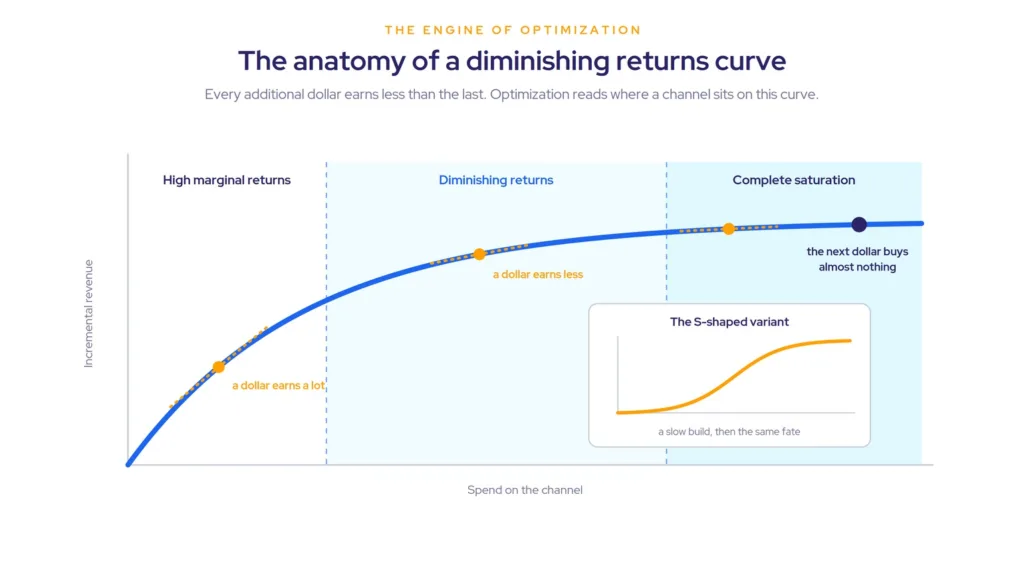
The whole exercise, then, is finding the channels that have reached saturation and moving their excess budget to the channels that still have room to grow.
Why ROI alone cannot decide the allocation
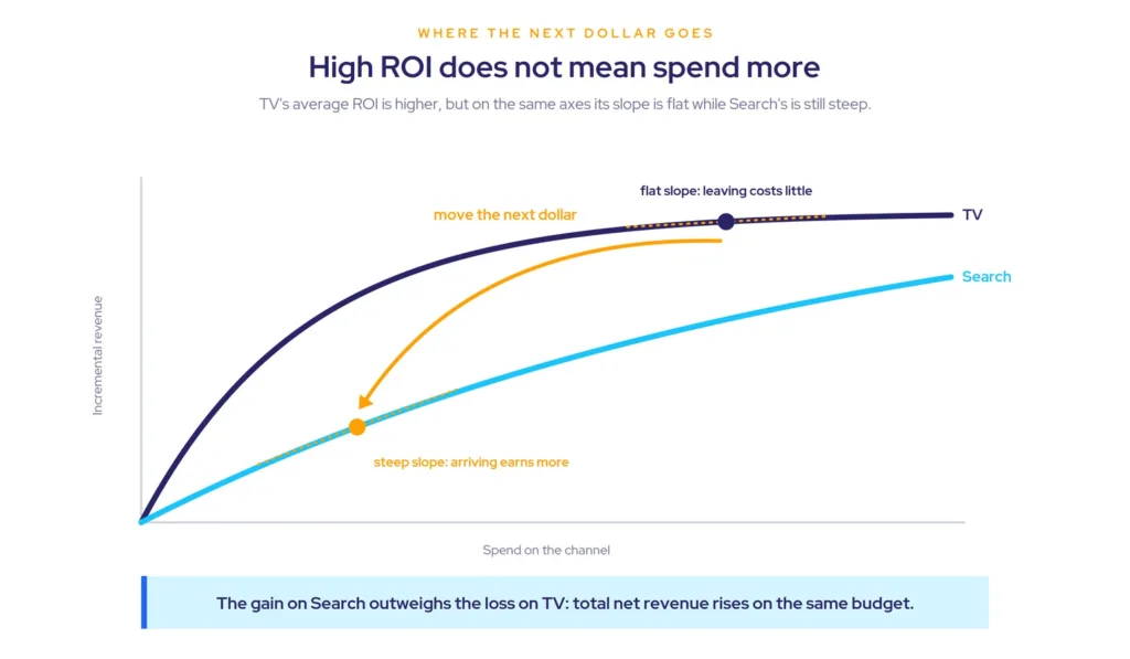
ROI is an average across everything a channel has already spent. Instead, the allocation question runs on the margin, on what the next dollar will do. Deciding where that next dollar should go takes both the ROI and the saturation level of every curve.
“A high ROI does not mean the business should invest more in that channel.”
For instance, take two channels, TV and Search, where TV has the higher ROI but sits close to saturation. Moving a dollar from TV to Search produces two effects. A small decrease in TV’s contribution, because its slope is flat. And a larger increase in Search’s contribution, because Search is not as saturated.
As a result, the gain on Search outweighs the loss on TV. Same total budget, higher total net revenue. In short, that mechanism is the whole of optimization. Everything else is scale and constraints.
A worked example: allocating $50k across three channels
To illustrate, say there is $50k to invest across three channels: CTV, Paid Social, and Retail Media. The first step is to derive the diminishing returns curve for each channel. The second is to split the budget into increments. In this example, $10k, $20k, and $20k.
“The optimizer never asks which channel performed best. It asks which curve is steepest right now.”
Iteration 1: the first $10k
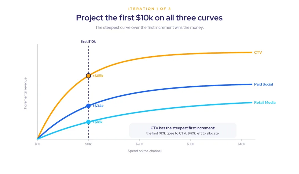
Project the first $10k on all three curves and compare the returns. CTV projects $65k of incremental revenue, Paid Social $34k, and Retail Media $18k. Since CTV has the steepest first increment, the first $10k goes to it.
After iteration one, CTV holds $10k, Paid Social and Retail Media hold nothing, and $40k remains to allocate.
Iteration 2: the next $20k
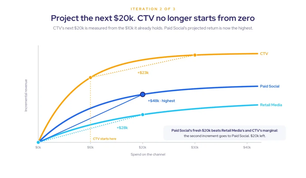
Project the next $20k on all three curves. However, one detail changes everything: CTV no longer starts from zero. Its projection is measured from the $10k it already holds, so the CTV curve now returns the marginal revenue of an additional $20k on top of that first increment. Comparing the three projected returns, Paid Social’s $48k is the highest, ahead of Retail Media’s $28k and CTV’s marginal $23k. The second increment goes to Paid Social.
Iteration 3: the last $20k
Likewise, the same procedure decides the final $20k, each channel measured from its current position. CTV would return a marginal $23k and Paid Social a marginal $8k, because both are projected from the spend, they already hold. Retail Media’s curve is still untouched, so its fresh $20k projection of $28k is now the highest. The last increment goes to Retail Media.
The final optimal allocation: CTV gets $10k from iteration one, Paid Social gets $20k from iteration two, and Retail Media gets $20k from iteration three. Notably, even the smallest channel earns its increment once the bigger curves have absorbed theirs.
In practice, real optimizers run this logic at much finer granularity and under real constraints: a total budget, a date range, and floors and ceilings per channel so the math respects contracts and inventory. MassTer Mind is built for exactly that job. The principle does not change.
Marketing mix optimization happens at several levels
Overall, optimization is not confined to a single view of the business. You can run it at several levels of the organization, depending on the decision in front of you:
- For a single brand or product
- For a portfolio of brands
- At the country level
- At the business unit level
- At the product category level
Additionally, a useful resource for going deeper on each approach is the book Marketing Payback by Robert Shaw and David Merrick, which covers the techniques in more detail.
A real-world example: reallocating away from a saturated channel
The clearest way to see this is on a real engagement. A major personal hygiene brand came to us with a media plan that looked healthy on the surface. Every channel showed a positive ROI, so nothing stood out as a problem.
The model told a different story. One of the brand’s largest channels was running at 96% saturation. Its average ROI still looked strong, which is exactly how an average hides the truth: the next dollar into that channel was earning almost nothing, even though the budget already spent there had earned well.
The optimization moved that trapped budget into channels that still had room on their curves. Same total spend, no increase in budget. Total media-driven revenue rose 5.5%. Nothing was added. The money was simply placed where the next dollar earned the most.
The effect compounds at portfolio scale. For a global retailer, reallocating across the full portfolio lifted media-driven revenue by about 18%, roughly $30 million, and moved marketing ROI from 13 to 15.5. The mechanism is identical, applied across many curves at once.
The recommended optimization process
Based on MASS Analytics’ experience running these projects, five steps make an optimization robust. Importantly, they happen during modeling, not after it.
Step 1: Apply variable transformations (AdStock, carryover)
Consumers rarely buy the moment they see a campaign, so there is a carryover effect to account for. Transformations like AdStock model it. In addition, some algorithms capture both the short-term and the long-term effect of advertising.
Step 2: Add diminishing returns functions
AdStock on its own is linear. It does not produce the concavity optimization requires, so we apply a functional form that does, the exponential function for example, on top of it. Some analysts prefer an S-shaped curve at this stage.
Step 3: Create multiple candidate curves
Varying the saturation parameter in the chosen function produces multiple candidate curves. In turn, each one represents a different saturation level to be tested at the selection stage.
Step 4: Apply a model selection algorithm
Selection is where we choose the right curve to go into optimization, weighing it against all the other factors in the model. In particular, the curves have to make sense on visual inspection, neither fully saturated nor entirely unsaturated.
“A curve that never saturates tells the optimizer to spend everything on one channel. No business signs off on that.”
A fully saturated curve has the opposite problem. It tells the optimizer to spend nothing there. Neither reflects reality. For this reason, curve construction belongs inside the modeling process rather than after it.
Step 5: Optimize the budget
Once we select the curves that best fit the data, they therefore feed into the optimization to allocate the budget, exactly as in the walkthrough above.
Common mistakes when optimizing marketing mix models
Forgetting the business perspective
Optimization is not an exercise for a closed room. Input from the business and the media planners is what makes the output implementable, because reality carries constraints the data does not show. A channel with limited inventory, for example, needs a ceiling on how much the optimizer is allowed to place there.
Asking the manager or the subject-matter experts is advisable. Indeed, they usually hold exactly the constraint knowledge the algorithm is missing, and this is one of the common failure points in MMM projects generally.
Not iterating enough
“Modeling and optimization are not sequential steps. Treat them as iterative or expect bad surprises.”
Here is how the sequential version fails. The team builds the model, reports ROI and contribution, and the business then asks for an optimization on top.
An optimizer faced with those curves does the only thing it can. Zero on the saturated channels, everything on the rest. Consequently, no business accepts that plan.
The fix is to keep an eye on the optimization results while the team is still building the model, and iterate until modeling, optimization, contribution, and ROI all make sense together. Thus, the project finishes only when all four agree, not before.
The software and tools behind optimization
Most open source MMM packages ship with a basic optimizer, but in our experience they lack what an accurate optimization process needs: real constraints, portfolio-level allocation, and a way to stress-test a plan before anyone commits to it.
MassTer Mind is built for exactly that. It is MASS Analytics’ no-code marketing budget optimization software, and it sits on top of a finished Marketing Mix Model rather than replacing it. By design it is model-agnostic, so it runs on any Marketing Mix Model, whatever platform built it, open source or proprietary.
Mind turns the model into a live planning and optimization engine. It allocates budget increment by increment across the curves, respects a total budget and floors and ceilings per channel so the math honors contracts and inventory, and lets you simulate a plan, layer in external conditions, and compare options before you commit. That final step, testing the allocation against the real world, is what turns the mathematically best answer into a decision a team can actually sign.
For single-product work inside the modeling environment, the same optimization engine is also available in MassTer Studio.
The backbone is the curve
According to MASS Analytics, the backbone of any marketing mix optimization exercise is the definition of the diminishing returns curves. In summary, transform the variables, apply the carryover, build in diminishing returns, create multiple sensible candidates, and use model selection to find the curve that deserves to drive the allocation.
The optimizers will keep getting faster. Ultimately, the teams that win the next decade will be the ones whose curves deserve the confidence the algorithm places in them. For the deeper practitioner view on reading the curves and deciding where the next dollar should go, see our companion piece, and for the full workflow behind these ideas, see our Comprehensive Marketing Mix Modeling Guide.
Further reading
For those who want to dig into the academic foundations, we recommend the following papers and talks:
- Practice Prize Winner, Dynamic Marketing Budget Allocation Across Countries, Products, and Marketing Activities, Marketing Science
- Optimizable and implementable aggregate response modeling for marketing decision support, ScienceDirect
- A New Theorem for Optimizing the Advertising Budget, the Journal of Advertising Research
- Creating Optimal Marketing Budget Allocation: With and Without Data, Marketing Science Institute
Frequently asked questions about marketing mix optimization
Optimization uses the diminishing returns curve of each channel, which modeling produces, to allocate budget increment by increment. Each increment goes to the channel whose curve is steepest at its current spend level, then the optimizer recomputes the slopes and repeats the process until it spends the whole budget. The result is the allocation with the highest total projected return under the constraints we set.
A diminishing returns curve maps spend on a channel to the incremental revenue it generates. The curve is concave or S-shaped: each additional dollar earns less than the one before, and at complete saturation the curve goes flat, meaning the next dollar buys almost nothing. In short, these curves are the backbone of any optimization exercise.
AdStock is a transformation that models the carryover effect of advertising, since consumers rarely buy the moment they see a campaign. AdStock alone is linear, so we apply a diminishing returns function on top of it to produce the concave shape optimization requires. Ultimately, skipping that step leaves the optimizer with curves it cannot allocate against sensibly.
We divide the total budget into blocks, and project each block onto every channel’s curve from that channel’s current spend level. The block goes to the channel with the highest projected marginal return, the positions update, and we project the next block again. Importantly, we measure channels that already hold budget from where they sit, not from zero.
Because optimization exposes curve problems the model statistics do not. If curves turn out fully saturated or entirely unsaturated only after the team reports the model, the optimizer will produce an allocation no business accepts, and the team has to redo the modeling. Checking optimization results during modeling catches this early, so the project is done only once both make sense together.
Two shapes disqualify a curve. One that never saturates, which tells the optimizer to pour the entire budget into a single channel, and one that is already flat, which tells it to spend nothing there. Neither reflects reality. Overall, curves should be concave or S-shaped with a visible but not extreme saturation level, which model selection chooses.