The Metrics You Need to Know in Marketing Mix Modeling

A MASS Analytics guide to the core MMM metrics: which one answers which question, and where each one misleads

Marketing Mix Modeling produces a lot of numbers. The skill is knowing which number answers which question, and where each one quietly misleads you. This guide walks through the core MMM metrics in the order a model actually uses them: from what drove sales, to how you value it, to how efficiently each channel converts spend, to where the next dollar should go.

Each metric answers a different question. They are read together, not ranked against one another.

Contribution

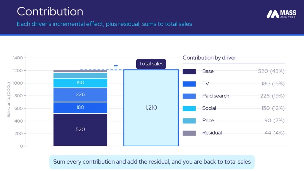
Contribution is the incremental impact of a single factor on your KPI. It can be expressed in absolute terms or as a share of total sales.

Say you model sales units and measure the contribution of paid search at 22,600 units. That means the search activity you invested in produced 22,600 additional units. Not correlated with them. Caused them, net of everything else in the model.

Contribution is what the whole decomposition is built from. Sum the contribution of every factor, add the residual, and you return to total sales. That reconciliation is the contribution chart.

Waterfall charts

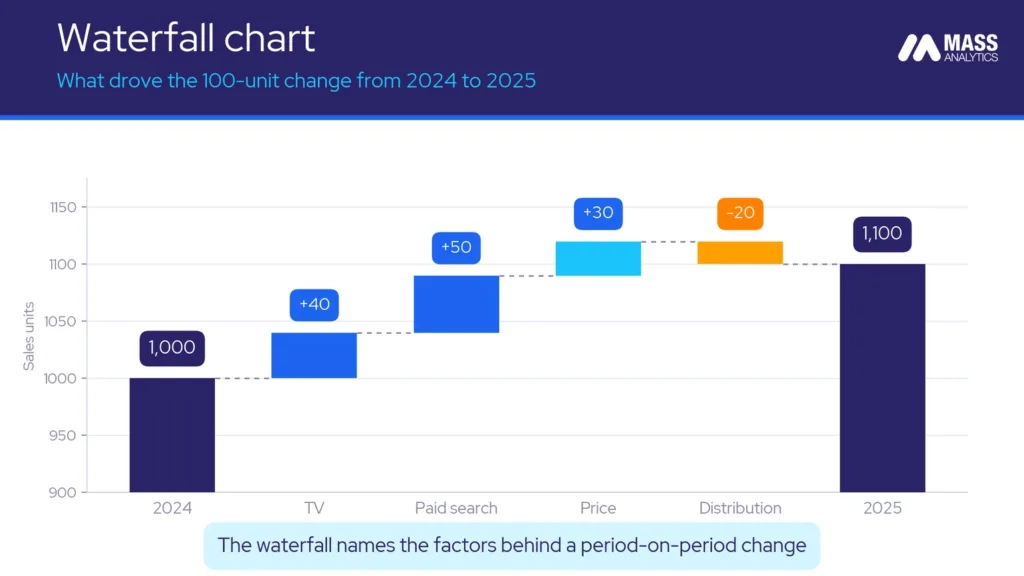
A waterfall chart reads contribution over time. It answers a specific question: what changed between one period and the next, and which factors are responsible.

Suppose you recorded 1,000 units in 2024 and 1,100 in 2025. That is a 100-unit increase. The waterfall breaks that increase into its parts, so you can see exactly which channels added units and which lost them. Add the movements together and you land back on the 100-unit change.

The same chart works in percentage terms. Divide each movement by the prior period’s sales, and the percentages sum to total growth.

Incremental revenue

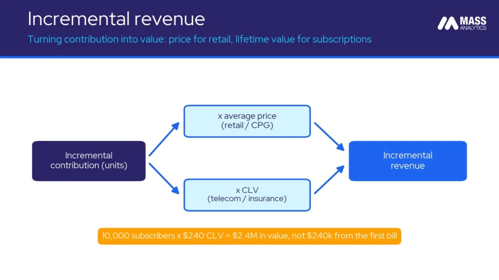
A media model usually produces contribution in units. To make it a business number, you convert those units into incremental revenue.

In consumer goods and retail, the conversion is direct: contribution in units times average selling price. Use weekly prices against weekly contribution where you have that granularity, then sum.

Subscription verticals break that logic. In telecoms, insurance, and banking, one acquired customer does not generate a single revenue event. They generate renewals and cross-sell over a contract. Treating the first transaction as the full impact understates ROI severely. The fix is to convert with Customer Lifetime Value:

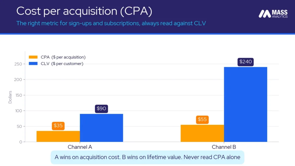
A telecoms brand that acquires 10,000 subscribers at a CLV of $240 generated $2.4 million in value from that spend, not $240,000 from the first month’s bill. That distinction changes the ranking of acquisition channels, and it changes how the budget is argued at board level. CLV comes from the finance or data science team, because it needs churn and renewal data.

Return on investment (ROI)

ROI is the ratio of incremental revenue to spend. It tells you how much revenue each dollar in a channel returned.

Both sides of that ratio have to be in money. When you model digital in impressions, or offline in GRPs, convert those back to spend for the denominator before computing ROI. Use the actual buying cost during the modeled period, not current rate cards.

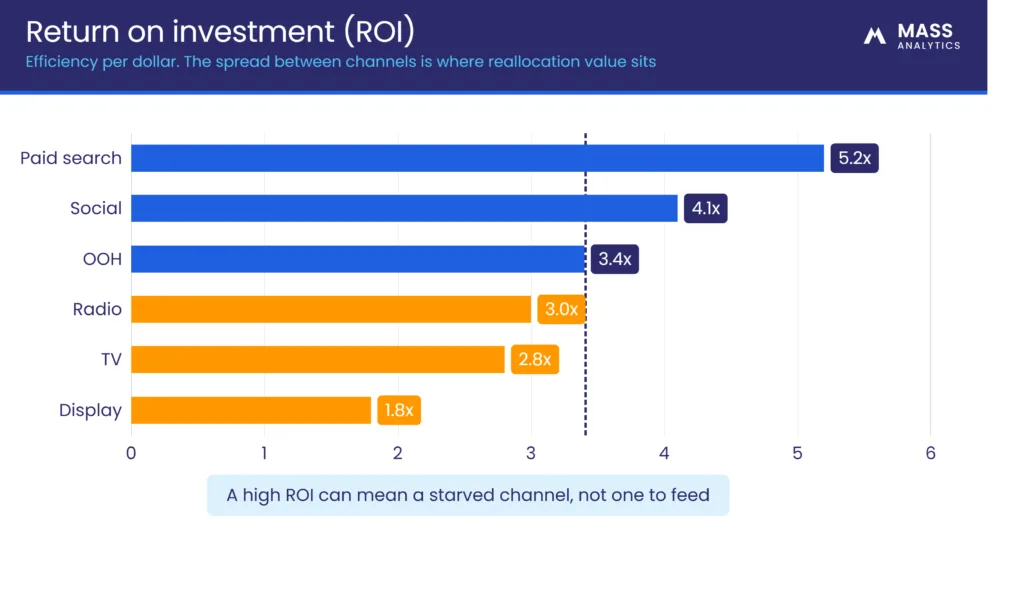
ROI is a measure of efficiency, not of scale. A channel at 4.0x returns four dollars per dollar spent. That says nothing about how much total revenue the channel generates, or whether the next dollar would also return four. Ranked across channels, ROI shows you where the spread is, and the spread is where reallocation value lives. Here is the trap. A high ROI often means a channel is spent at a low level, well below saturation, not that it can absorb more at the same return. Push more spend in and you move up the response curve, where each dollar returns less. So a high ROI can be the signal of a starved channel, not a channel to feed. The decision of where the next dollar goes is governed by marginal return, which we come to below.

Cost per acquisition (CPA)

When the objective is a discrete action, a sign-up, a subscription, a lead, or a download, CPA is the more useful efficiency metric. It measures what it costs to generate one of those actions.

CPA earns its place when the sales cycle is long and revenue lags the campaign by weeks or months, which makes revenue-based ROI impossible to compute at review time. It is common in financial services, telecoms, gaming, and subscription platforms.

Never read CPA alone. A low CPA that brings in low-value customers can produce a worse lifetime ROI than a higher CPA that brings in high-value ones. Read it against CLV every time.

Effectiveness

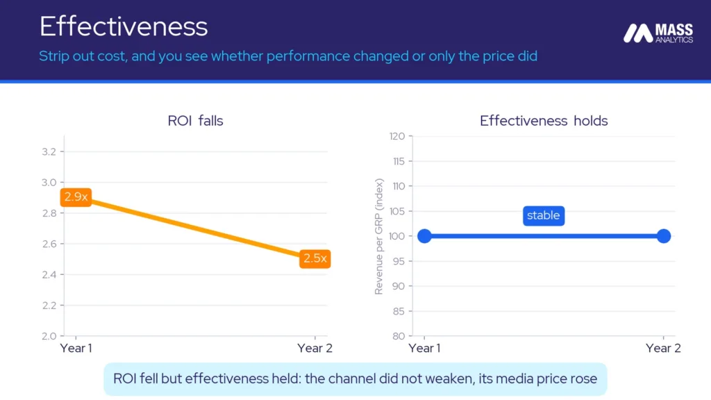
ROI can move for a reason that has nothing to do with performance: the price of media. Effectiveness is the metric that separates the two.

It replaces spend in the denominator with the underlying media unit, so cost inflation drops out.

Now the diagnosis is clean. If ROI fell year on year but effectiveness held steady, the channel is converting exposure at the same rate it always did, and the ROI drop is a media price story. Negotiate the rate. Do not cut the budget. If ROI and effectiveness fell together, that is a genuine performance problem, and the response is an execution review.

Efficiency index

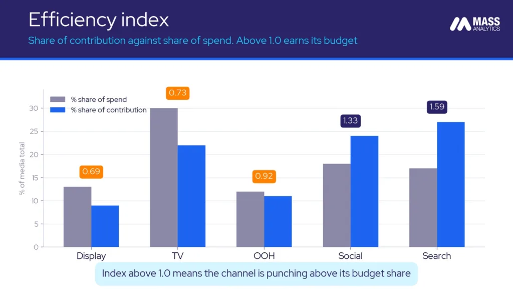
Effectiveness looks at one channel over time. The efficiency index takes a portfolio view. It compares a channel’s share of total media contribution to its share of total media spend.

An index above 1.0 means the channel delivers more than its budget share, so it is punching above its weight. Below 1.0 means it is absorbing more budget than its contribution warrants. This framing lands well with media agency teams, whose planning is share based rather than ratio based.

One caution. Always check the response curve before acting on an efficiency signal. A high-efficiency channel sitting near saturation will lose that advantage quickly if you add spend.

Diminishing returns

The backbone of any optimization exercise is the diminishing returns curve. It plots the relationship between spend on a channel and the incremental revenue that spend produces.

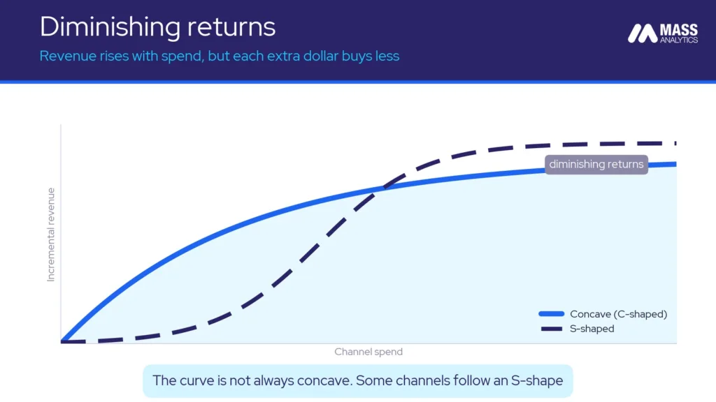
The relationship is not linear. It is concave: the more you spend, the more revenue you get, but at a slower and slower pace. As spend climbs, you hit diminishing returns, and additional revenue becomes hard to buy.

The curve is not always concave from the origin. Sometimes it is S-shaped, with an early convex region of increasing returns, then a concave region of diminishing returns. The shape matters, because it decides how the optimal spend zone is defined, as we will see.

Marginal returns

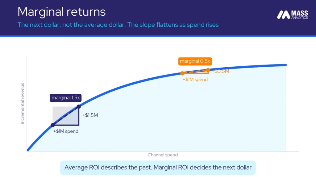
Marginal return is the revenue from the next dollar, not the average dollar. It is the slope of the response curve at your current spend level.

Early on the curve, one million dollars of spend might return 1.5 million in revenue. Later, at higher spend, that same one million returns only half a million. The impact per dollar falls as you move up the curve, until the channel reaches saturation and further investment stops being worthwhile.

That gap between the early dollar and the late dollar is the whole point. Average ROI tells you how spend has performed in aggregate. Marginal ROI tells you what the next dollar will do. Only one of them should drive a reallocation decision, and it is the marginal one.

Optimal execution range

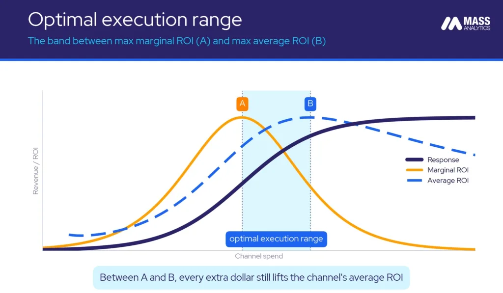
The optimal execution range is the spend band within which a channel produces its most efficient marginal return. It only exists on an S-shaped curve.

It is bounded below by the spend level where marginal ROI peaks, call it Point A, and bounded above by the spend level where average ROI peaks, Point B. Between those two points, every additional dollar raises the channel’s running average ROI, because the marginal return on that dollar is still higher than the average. Past Point B, the marginal return falls below the average, and the channel’s average ROI begins to decline. The band from A to B is the productive zone: the range where more spend is unambiguously efficient.

On a concave curve there is no Point A, because marginal ROI is highest at the very first dollar and falls from there. In that case the optimal zone comes from the profit curve instead, running to the point where marginal profit reaches zero.

One reminder before you act on any of this. Optimization is a portfolio exercise, not a channel-by-channel one. The optimal range for a single channel is only the input. Where the money actually goes depends on every channel’s range at once.

Frequently asked questions

Core definitions

Reading ROI correctly

Applying the metrics