In the previous part of this MMM Guide series, we explored one of the corner stones of Marketing Mix Modeling, which is Regression Analysis. In this article we cover some of the ways in which you can ensure the robustness of your model and reliability of your results. This step is very important and should be performed at the modeling stage of the MMM workflow. Now that you have built a marketing mix model that makes sense, how do you make sure it’s statistically sound?
There are a number of tests you need to conduct to be sure. Here are the key statistics that should be computed and analyzed to evaluate the robustness of your marketing mix model.
1. R Squared: How much Variance is explained by the model
The coefficient of determination, or R Squared for short (often referred to as R², measures the percentage of the total variance that is explained by the model. For example, if R squared is equal to 85%, it means that 85% of the variance in the Sales data is explained by the variables in the model e.g. media promotions, distribution, seasonality etc.. A modified version of the R² is the adjusted R². One of the drawbacks of the R² is that it increases as the number of variables in the model increases regardless of their explanatory power. The adjusted R-squared on the other hand only increases when the new variables added to the equation improve the model more than what would be expected by chance. It also decreases when a predictor/independent variable improves the model by less than expected. Adjusted R Squared is often used to compare the explanatory power of two models.
2. F Statistic: Overall Model Relevance/Significance
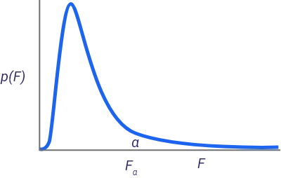
The F test measures the overall significance of the model. H0 that is related to this F test, states that all the coefficients are equal to zero at the same time.
Taking the same example (if R squared is equal to 85%, it means that 85% of the variance in the Sales data is explained by the variables in the model e.g. media promotions, distribution, seasonality etc..), the test is to see whether all the coefficients of media, promotions, seasonality, and distribution (i.e all the variables in the equation) take zero at the same time.
If this is the case, it means that overall, the model is not significant and none of the variables seem to impact the dependent variable significantly. If the F test turns to be significant, then you need to proceed and test every single variable separately and statistically. Be aware though that rejecting H0 of the F stat does not mean that every single variable in the equation is significant.
3. T-Statistic: Relevance Significance of one predictor
The t-stat is a measure of coefficient reliability. It is the ratio between the computed (or the estimated) coefficient and the standard error of the coefficient.
The bigger the t-stat the better, as it means the coefficient is statistically different from 0 (0 indicates absence of relationship between the dependent and the independent variable). In other terms, if another sample is drawn, it is likely to obtain a similar or close measure of the coefficient and that value is ensured to be different enough from 0.
The t-stat is computed for each independent variable in the equation. So as a rule of thumb, if the t value of a variable (search for example) is greater than two, then the variable is statistically significant and search has a significant impact on sales.
4. The Standard Error of The Estimate (SEE) and the MAPE: Model Accuracy
This statistic is an average error of all the residuals that have resulted from the model creation. This metric should be as small as possible because it means that overall, the error (difference between the real value and it model estimate) throughout the different data points is controllable and of a small size.
The MAPE or Mean Absolute Percentage Error is also a measure of prediction and model accuracy, hence the smaller the merrier.
MAPE is computed as the average of the individual absolute forecast errors divided by the actual values for each period: it is the mean of the relative percentage of errors. The closer the MAPE value is to zero, the better the predictions.
It has the advantage of presenting the error in percentage units instead of the variable’s units.
5. Durbin Watson: Checking for Autocorrelation
Durbin-Watson (DW) is used to test whether the residuals of the model are independent of one another.
Autocorrelation is one of the assumptions of the OLS estimation method This statistic varies between 0 and 4. A value of 2.0 indicates the absence of autocorrelation.
6. The Variance Inflation Factor: Checking for Multicollinearity
The Variance inflation factor, or VIF for short, indicates whether the explanatory (independent) variables are correlated.
In regression analysis, the VIF statistic should be under five for every single variable. If it is not the case, it signals that there is a multicollinearity problem.
Multicollinearity is one of the most challenging issues in MMM projects. In fact, brands tend to deploy several channels at the same time, especially the digital ones (search, display YouTube..).
This results into multicollinearity problems and difficulties in disentangling the impact of each channel.
7. Jarque Bera, Kurtosis, Skewness: Checking for Normality
Jarque Bera, kurtosis, skewness, and others are different ways to test the normality of the residuals. The latter should be normally distributed.
It’s Not Just About Statistics, Think About the Business Story Too!
Establishing that a model makes sense statistically is crucial. But that is only one half of the story; MMM is about modeling consumer behavior, hence it is also crucial that the model makes commercial and business sense. For example:
- When modeling a CPG brand, it is not possible to accept that price has a positive impact on sales. One cannot present results that say: the higher the price, the higher the sales. That is counter intuitive.
- If a business is spending $20 million on advertising, and the model says that the advertising coefficient is negative, then they need to re-evaluate their model to see if they made the right transformations.
Not only should you take the time to evaluate the equation from a statistical standpoint, but you should also assess whether the level of elasticity, seasonality, ROI, and the different parameters that you are estimating make sense business-wise. You should be able to seamlessly defend them when presenting the results back to the client or your internal team.
Modeling is an iterative process. You will often find yourself going through multiple models before you are finally satisfied with the results you’re getting. With rigorous model evaluation, you can be confident you are on the right track in your marketing mix modeling journey!
R Squared
OR
Adjusted R Squared
OR
k denotes the number of independent variables (k=p-1)
F Statistic
where
Testing the Overall Significance of the Regression (F-Test)
H0:not all the parameters are 0
So if Fcal > Ftable reject H 0
We can calculate an Fcal value from the of value of R Squared

T-Statistic
The Standard Error of the Estimate
Simple Regression Model
The Standard Error of the Slope
The Standard Error of the Regression
Multiple Regression Model
The Standard Error of the Regression
The Standard Error of the slope
MAPE
Durbin Watson
The Variance Inflation Factor
Jarque Bera


Model Statistics in MassTer
With MassTer, you can evaluate your model using various statistics. When building and tweaking your model, these statistics will be instantaneously updated and displayed on a table above your model.


