Imagine you’re the CEO of an ice cream company. You have the best-selling ice cream in the nation. Very tasty stuff!
One day, you notice your sales numbers dropping. You look at the possible suspects but you’re not seeing an obvious reason for the decrease. You look for a way to understand exactly what’s driving your sales. Being the savvy CEO that you are, you commission a Marketing Mix Modeling project to get to the bottom of it. Your marketing analytics team gets to work and comes up with an initial model about the sales of your beloved ice cream. It looks like this:
Where:
Y: ice cream sales
x1: price
x2: distribution
x3: temperature
There are immediate problems with this model. In the real world:
If the price is zero: sales are expected to be infinite in the sense they would keep buying indefinitely, assuming stock is available. However, looking at this equation, if the variable that is related to price is replaced by 0. The number of sales will be a finite amount of sales, which is counter-intuitive.
If the distribution is zero: sales should be zero as the product cannot be sold. This is not the case in this equation. Actually, if the distribution is replaced by zero, there will still be some sales.
If the temperature significantly decreases to negative degrees Celsius, the sales cannot become negative.
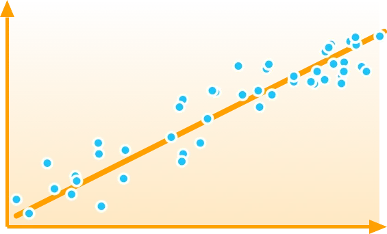
This equation does not really help your analysts understand and model how consumers behave in real life. It is a case where linear models fail.
So what can you do instead? Use log-linear.
What is Log-Linear Modeling
A log-linear model is a multiplicative model that is composed of two main categories of variables:
Relative variables (like distribution and price)
Incremental variables (like promotions, TV, media, etc.)


Defining Relative & Incremental Variables
MassTer provides possibility of Defining the type of variable you are working with (relative/incremental). This can be done in the Configure module by double clicking the variable group desired in the describe tab. Group parameters will be applied on all the variables added to the group, so make sure you have the right variable in the right group.
⇒ Change the Group Type to: Incremental/ Relative
Take this equation as an example of a log-linear model:

When the distribution is equal to zero, sales will be equal to zero. That is what is expected in real life. Similarly, if the price is equal to zero, sales will be infinite. In other words, log-linear is capable of better mimicking reality than linear regression. Therefore, modeling using log-linear is preferred to modeling using just simple additive formulations.
Building a Log-Linear Model
To estimate the Log-Linear model, you must first estimate the coefficients to report on the impact of the different factors, whether they are relative or incremental.
Then, you apply log to both sides of the equation to obtain a linear model:
Linearization
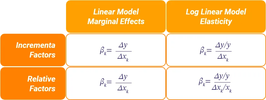
Coefficients are then estimated using Ordinary Least Squares (OLS). Interpreting the coefficients would depend on their type:
For relative variables: the coefficient depicts elasticity, which is very beneficial to have.
For incremental variables: the coefficient depicts the percentage change in the dependent variable as a result of one unit change in the incremental variable, for example, TV, display, search, and even promotion.

Limitations of Log-Linear
The problem with using log-linear for MMM is that businesses expect their teams to report on the contribution of each media and marketing activity. However, the multiplicative form of the log-linear makes it very difficult to separate contributions.
That is why approximation approaches are used to transform the multiplicative model into a summation where the individual contribution of every variable is clearly distinguished:
Obviously, this is an approximation that will result in a decomposition error. The latter will be added to the standard OLS error:
Remember, any algorithm that claims to approximate contribution in the context of log-linear needs to make sure that the decomposition error is as small as possible.

