
Dr. Ramla Jarrar of MASS Analytics explains Bayesian marketing mix modeling: how priors work, when Bayesian beats OLS, MCMC vs MAP, and how experiments calibrate your MMM.
- →The claim every modeling approach makes about where knowledge lives
- →Three prior types, and the coefficient of variation settings that control them
- →Four data conditions where Bayesian regression outperforms OLS
- →The experiment-to-prior calibration loop, and where its critics have a point
- →MCMC, MAP, and Empirical Bayes compared, plus the failure modes vendors leave out
Bayesian marketing mix modeling starts from a premise many measurement teams find uncomfortable: your data does not know everything about how your marketing works. Your team does. Classical regression lets the data speak alone. Bayesian regression starts with what you already know, updates it with what the data shows, and produces an answer that reflects both. When budgets run thin, channels correlate, or a category turns noisy, that combination determines whether your model survives scrutiny. Ultimately, it is the difference between a measurement you can defend and one that collapses under the first serious question from the CFO.
The methodology is having a moment. Google’s Meridian, PyMC-Marketing, and Meta’s Robyn have pushed prior-driven modeling into the standard MMM toolkit. As a result, every vendor deck now carries a Bayesian slide. I have watched this industry through enough hype cycles to be careful here. The industry once presented multi-touch attribution as the future of measurement, too. So here is the honest position instead. Bayesian regression solves specific problems that classical regression handles poorly, and those problems arise regularly in real MMM programs. In the wrong conditions, however, it will make your measurement worse, not better.
When channels are correlated and budgets are thin, letting the data speak alone is not rigor. It is waste. Bayesian MMM formalizes what your team already knows instead of throwing it away.
Every modeling approach makes a claim about where knowledge lives
Classical OLS regression says knowledge lives entirely in the data. Give it a rich, varied sample and it will find the parameters that best explain the relationship between media and sales. Give it a short history, a noisy category, or highly correlated channels, however, and it will struggle. The symptoms are familiar: unstable estimates, wide confidence intervals, and coefficients that flip when you add or remove a single variable.
Bayesian regression says knowledge lives in two places: the data, and everything you knew before you saw the data. You start with a prior distribution for each parameter, a formal statement of what a plausible value looks like based on previous models, experiments, and commercial experience. The data then updates that belief. The result is a posterior distribution: what you now believe, given both sources of evidence.
Bayes theorem sounds intimidating and is not. In plain language: what I now believe about a channel’s ROI is a weighted combination of what I believed before modeling and what the sales data shows. When the data is rich, it dominates and the result looks like OLS. When the data is thin, the prior carries more weight and keeps the estimate commercially grounded.
One more difference matters in the boardroom. A Bayesian model does not say “the TV ROI is 2.3.” It says there is an 85% probability that the TV ROI lies between 1.6 and 3.2. We call that range a credible interval, and it is more honest than a point estimate. The foundations of regression analysis for MMM apply to everything that follows here.
The prior is the most consequential choice in the model
Get the prior right and the model produces stable, commercially grounded results even when the data is noisy. Get it wrong and the model produces results worse than OLS, because the prior has anchored the estimates in the wrong place. In short, everything else in Bayesian MMM is machinery. This is the decision.
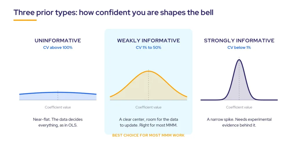
Priors come in three strengths. An uninformative prior is nearly flat: the model assumes you have no opinion, the data decides everything, and the result looks like OLS with extra compute. A weakly informative prior has a clear center but a wide spread: you have a point of view, and the data is free to revise it. A strongly informative prior is a tight spike around a well-evidenced value: it will shape the result even when the data disagrees, so it demands experimental justification.
The coefficient of variation, the standard deviation of the prior divided by its mean, controls the width of each of those bells. Below roughly 1%, the prior dominates. Between 1% and 50%, prior and data share influence, which is the right setting for most commercial MMM work. Above 50%, the data dominates and you have given up most of the stabilization benefit.
Where should priors come from? The best source is your own measurement history. The posterior from the last model becomes the prior for the next, and each successive model carries the accumulated learning of all previous ones. The second best source is controlled experiments, which I will come back to. The worst source, and the most common one, is an unexamined benchmark or a stakeholder’s intuition formalized without challenge.
One practice I insist on with every client: review the priors with the business before the model runs. Show the marketing director the proposed ranges. Ask whether they believe them. A prior that surprises the marketing team in the results meeting is one nobody consulted them on, and it creates a credibility problem no amount of posterior precision can fix.
The prior is the most consequential choice in a Bayesian model. Well-sourced priors stabilize noisy data. Poorly sourced priors anchor the model in the wrong place and produce results worse than OLS.
Four conditions where Bayesian MMM outperforms classical regression
The first is collinearity. Teams typically plan TV and online video budgets as a fixed ratio, producing correlations of 90 to 95%. At that level, OLS estimates swing wildly between model runs. A Bayesian prior anchors each coefficient within a plausible commercial range and expresses the remaining uncertainty honestly, as a wide credible interval, rather than hiding it in unstable point estimates.
The second is thin data. Classical MMM wants two to three years of weekly history. Bayesian regression produces useful results on shorter histories, for new product lines, small channels, or fast-moving categories, because the prior fills in with what the team knows from adjacent products and comparable markets. This does not invent information. It formalizes knowledge you already have instead of discarding it.
The third is update stability. In a classical program, every refresh re-estimates from scratch, and a TV ROI that moves 30% between quarterly updates will destroy boardroom confidence in the measurement system. In a Bayesian program, the posterior from the last run is the prior for the next. The model learns incrementally, and results move only when the evidence moves.
The fourth is planning under uncertainty. Because the output is a distribution, the optimization can produce a range of credible budget plans, each with its expected return and its variance. A business growing aggressively can pick the high-variance plan. A business defending share can pick the narrow one. That choice belongs to the planning team, and a point estimate takes it away from them.
I have seen all four conditions land at once. A global automotive brand we worked with needed to allocate budgets across vehicle nameplates, regional markets, and two media tiers, with linear and addressable TV heavily correlated. A Bayesian hierarchical structure, with priors carried from previous model generations, stabilized the nameplates that had thin current data. It also confirmed a reallocation from linear TV to addressable in the markets where marginal returns were higher. The same partial pooling logic drives hierarchical modeling in the classical framework; Bayesian estimation extends it with explicit prior beliefs.
Be equally clear about the reverse case. With a rich data history, strong independent channel variation, no reliable prior evidence, and a fast turnaround requirement, OLS is simpler and faster. In fact, it produces similar results under those conditions. I made this argument at length in Regression Is Not Stuck in 1995. Neither approach is universally superior. The data conditions decide.
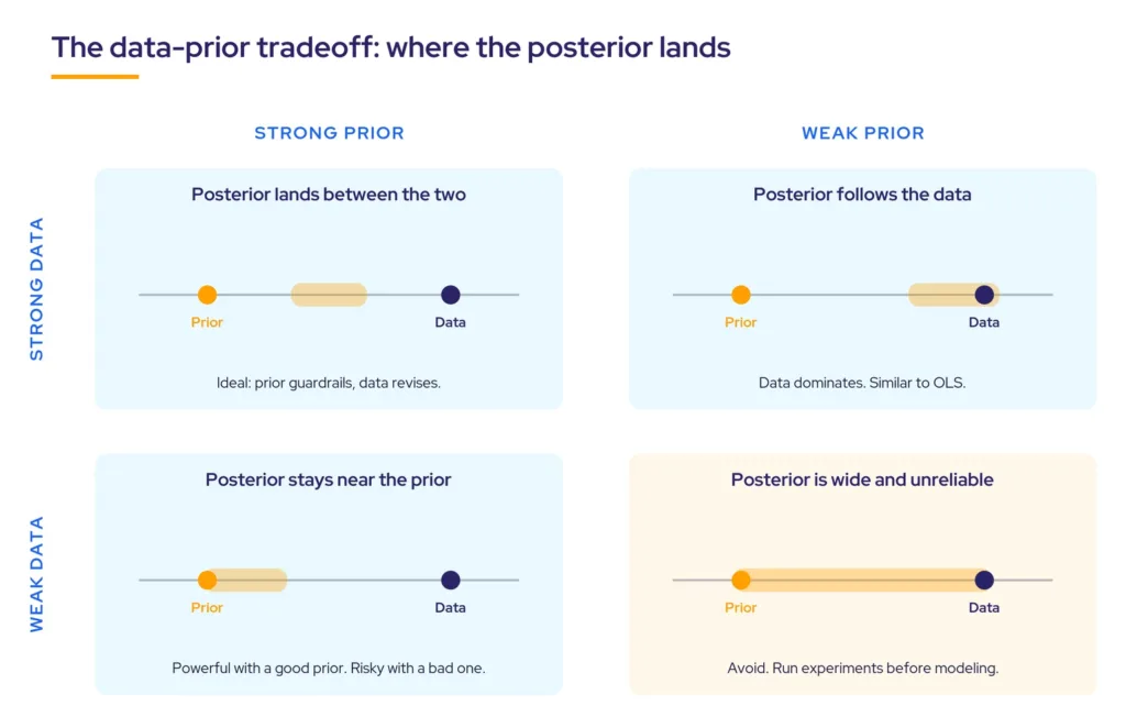
A Bayesian model in the wrong hands, built on poorly designed priors, will produce results less reliable than a well-specified classical model. No package changes that.
Here is the full comparison in one view.
| Dimension | Classical OLS regression | Bayesian regression |
|---|---|---|
| Core assumption | Parameters are fixed unknowns; the goal is the single best estimate from the data. | Parameters are distributions; the goal is the full range of plausible values given prior and data. |
| Prior knowledge | Incorporated informally: variable selection, feature engineering, and parameter constraints applied by the modeler across iterative runs. | Incorporated formally as prior distributions with documented sources; auditable and carried between runs. |
| Output | A point estimate per coefficient, with a confidence interval. | A posterior distribution per coefficient, summarized as a credible interval. |
| Data requirement | Two to three years of weekly history for stable estimates; struggles with short histories and correlated channels. | Works on shorter histories; the prior stabilizes estimates where data is thin or channels are correlated. |
| Model updates | Each refresh re-estimates the coefficients; consistency between runs depends on the modeler’s discipline. | The last posterior becomes the next prior; updates are incremental by construction. |
| Uncertainty | Confidence interval: a statement about repeated sampling, often misread in the boardroom. | Credible interval: a direct probability statement, easier to use for planning decisions. |
| Speed and expertise | Fast, simple, widely understood by analysts and reviewers. | MCMC is slow and needs convergence diagnostics; MAP and Empirical Bayes trade posterior richness for speed. |
| Preferred when | Rich, varied data; independent channel variation; no strong prior evidence; fast turnaround. | Correlated channels; thin or noisy data; strong prior evidence from experiments or previous models. |
Experiments and Bayesian MMM cover each other’s blind spots
The most powerful application of Bayesian MMM is not the statistics. Rather, it is the loop it creates between measurement and experimentation. The model tells you which coefficients carry the most uncertainty. Those channels become your next experiments, designed with the model’s guidance on duration, test and control structure, and how much spend variation you need for a detectable signal. The experiment produces a causal lift estimate. That estimate becomes the prior for the next model run. Each cycle, the model gets better informed and the experiment budget gets better targeted.
A major airline’s model had carried an uncertain display advertising coefficient for years, because display generates exposure but few direct clicks. A three-month randomized controlled trial with device-level matching settled it. Specifically, 5% of e-commerce conversions in the exposed group were causally attributable to display that generated no click at all. The team adjusted the display coefficient by 22% and formalized the calibrated value as the prior for every subsequent run. One experiment, carried forward permanently.
The loop also works from zero. A brand with no TV history cannot model TV. Instead, one measurement team used their MMM to design a TV experiment: valid test and control regions, sufficient duration, enough variation to detect lift. The result became the prior for their first Bayesian TV coefficient. That brand now invests over $100 million a year in TV in the US on the strength of a measurement program that started with no data at all.
Some in the industry argue that experiment calibration inverts the logic of MMM: that it treats platform-friendly experiments as ground truth and forces the model to agree. The concern is legitimate when teams calibrate by brute force. It dissolves, however, when they treat priors as evidence to interrogate rather than instructions to obey. In one retail program, we used experiment results to set upper and lower bounds on a coefficient rather than a point value. As a result, the model kept the experiment’s causal validity without being forced into a number that ignored the rest of the portfolio. Calibration done that way strengthens the model. I have written about how incrementality measurement makes your MMM sharper and how incrementality testing closes the causal gap if you want the experimental side of the loop in full.
Run the experiment where the model is least certain. Feed the lift estimate back as a prior. Each model run makes the next experiment smarter, and each experiment makes the next model stronger.
MCMC, MAP, and Empirical Bayes are three routes to the same posterior
Full Bayesian estimation via Markov Chain Monte Carlo samples the entire posterior distribution. It gives the richest picture of uncertainty, and it is what most open-source packages run. That is why a Meridian or PyMC-Marketing model can take hours and requires convergence diagnostics before you trust it. R-hat below 1.1, posterior predictive checks, the full checklist. These are tasks for the modeling team, but they add real time and expertise requirements to the program.
Maximum A Posteriori estimation, MAP, finds the single most probable value instead of sampling the whole distribution. It is dramatically faster, which matters when your planning cadence expects refreshed results monthly rather than quarterly.
Empirical Bayes via expectation-maximization is the third route, and it is the one we implement in MassTer Studio, our modeling engine. You define the form of the prior, and the algorithm iteratively estimates the precise hyperparameter values from the data. This approach reduces the most dangerous risk in the whole methodology, a badly specified prior quietly biasing the model, while keeping the stabilization benefits that make Bayesian regression worth running.
One interpretation shift catches every classically trained analyst: in a Bayesian model, the t-statistic tests the posterior against the prior, not against zero. Significance means the data moved your belief, not that the channel matters. Therefore, brief your team before the first results meeting, not after.
A note on the tools, because the labels get blurred in vendor conversations. Google’s Meridian and PyMC-Marketing are Bayesian frameworks built on MCMC sampling. Meta’s Robyn takes a different route, regularized regression with evolutionary hyperparameter search, and is not fully Bayesian in the prior-to-posterior sense. All three are serious tools. None of them removes the need for statistical expertise, business understanding, and well-sourced priors. The tool is one part of the story, never the whole of it. Being open source, in fact, does not settle the trust question either. I made that longer argument in Transparency Was Never About the Source Code.
The failure modes nobody puts in the sales deck
The most dangerous failure in Bayesian MMM is not a model that looks wrong. It is a model that looks plausible on top of priors nobody ever interrogated. An unverified industry benchmark, a coefficient borrowed from a different category, an executive’s intuition dressed up as a distribution: any of these will anchor the model somewhere defensible-sounding and false. Every prior needs an explicit source, and that source deserves the same scrutiny as any other model input.
The second failure is stabilizing the wrong story. The same mechanism that makes Bayesian updating valuable, carrying results forward, will also propagate a past bias into every future run. If a channel’s true performance has genuinely shifted, a strong prior will dampen the signal. As a result, the model will look stable precisely when it should be revising. The diagnostic is simple and non-negotiable: check how far each posterior has moved from its prior at every refresh. A large shift means the data is telling a different story than the prior believed. Investigate before you present.
The third failure is communication. A boardroom trained on “the TV ROI is 2.4” does not immediately know what to do with a credible interval. Present the range as a planning guardrail, not as a confession of doubt, and use it consistently for scenario decisions. Reverting to a single number to look precise throws away the honesty you paid for.
Fit statistics detect none of these failures. Instead, validation discipline catches them — the same three layers of MMM validation that apply to any model: statistical soundness, commercial coherence, and external evidence.
Frequently asked questions about Bayesian marketing mix modeling
-
What is Bayesian marketing mix modeling?
Bayesian marketing mix modeling is an MMM approach that combines prior knowledge, formalized as probability distributions, with observed media and sales data. Instead of estimating each channel’s effect from the data alone, the model updates prior beliefs with the evidence and returns a posterior distribution: a range of plausible values for each coefficient, with an associated probability, rather than a single point estimate.
-
Is Bayesian MMM more accurate than traditional MMM?
Not universally. Bayesian MMM outperforms classical OLS regression when channels are highly correlated, data histories are short or noisy, or reliable prior evidence exists from experiments or previous models. With rich, varied data and no strong prior knowledge, OLS typically produces similar results faster. Accuracy depends on prior quality: a poorly sourced prior makes a Bayesian model less reliable than a well-specified classical one.
-
How much data does Bayesian marketing mix modeling need?
Less than classical MMM, which typically wants two to three years of weekly data for stable estimates. Bayesian regression can produce useful results on shorter histories because the prior compensates for thin data, drawing on adjacent products, comparable markets, or experiment results. It does not create information; it formalizes existing knowledge to stabilize estimates that OLS would return as highly uncertain.
-
What are priors in MMM and where should they come from?
A prior is a probability distribution expressing what a plausible value for a model parameter looks like before the data is observed. The strongest sources are your own previous model runs, where each posterior becomes the next prior, and controlled experiments that produce causal lift estimates. Unverified industry benchmarks and unchallenged stakeholder intuition are the weakest sources and the most common cause of misleading Bayesian models.
-
What is the difference between MCMC and MAP estimation?
MCMC, Markov Chain Monte Carlo, samples the entire posterior distribution, giving full uncertainty quantification at significant computational cost and requiring convergence checks such as R-hat. MAP, Maximum A Posteriori, finds only the single most probable parameter value, running far faster. Both use the same priors and data. MCMC suits deep uncertainty analysis; MAP suits programs that refresh models on a regular planning cadence.
-
Are Google Meridian and Meta Robyn Bayesian MMM tools?
Google Meridian and PyMC-Marketing are Bayesian frameworks: they specify priors and estimate full posterior distributions through MCMC sampling. Meta’s Robyn is not fully Bayesian; it combines regularized ridge regression with evolutionary hyperparameter optimization. All three are credible open-source tools, and none of them substitutes for statistical expertise, business understanding, and well-sourced priors.
Knowledge that compounds is the real return
Your data tells you what happened. It does not tell you what your brand knows, what your experiments have shown, or what a decade of measurement work has taught your team. Good classical modelers have always found ways to bring that knowledge in: through variable selection, feature engineering, and the constraints they place on parameters across iterative runs. What Bayesian regression changes is the form that knowledge takes. It moves from the modeler’s judgment, informal and hard to audit, into the model itself. Specifically, it becomes explicit distributions with named sources, where each posterior becomes the next prior and the learning compounds in a way anyone can inspect. Over years, that becomes a measurement asset that cannot be bought off the shelf and does not walk out the door when a modeler does. If you want the foundations under everything discussed here, our Comprehensive MMM Guide covers the full modeling arc.
So here is the question to take into your next measurement review. What did your team know before this model run, and where is it written down?
Marketing measurement knowledge should compound. Classical modelers carry it forward through specification and feature engineering. Bayesian MMM makes that carry-forward explicit, auditable, and quantified.
- ✓The prior is the decision that makes or breaks Bayesian MMM: well-sourced priors stabilize noisy data, and poorly sourced priors produce results worse than OLS.
- ✓Bayesian marketing mix modeling combines what your team already knows with what the data shows, returning a credible interval for each channel instead of a falsely precise point estimate.
- ✓Bayesian regression outperforms classical OLS in four conditions: highly correlated channels, thin or noisy data, programs needing stable incremental updates, and planning that can act on explicit uncertainty.
- ✓The experiment loop is the compounding asset: uncertain coefficients direct the next experiment, and each lift result returns as the prior for the next model run.
- ✓MCMC, MAP, and Empirical Bayes are different routes to the same posterior; choose the machinery your team can run correctly at your planning cadence.