
MASS Analytics explains how pooled regression measures sales across regions, stores, and retailers in Marketing Mix Modeling, why normalization keeps the results honest, and where hierarchical Bayesian methods now fit alongside pooled OLS.
- •What pooled regression is, and how it combines cross-sectional and time-series data
- •Why pooling multiplies the dataset and strengthens every regional estimate
- •The normalization problem that can reverse the sign of a coefficient
- •When to split variables to capture different regional sensitivities
- •Where partial pooling and hierarchical Bayesian methods fit next to pooled OLS in 2026
National models cannot answer regional questions
Marketing Mix Modeling at the national level treats sales as a single series and asks one question: what moved the total. That works until the question becomes regional. A retailer wants to see sales store by store. A consumer goods brand wants to compare performance region by region. Once measurement has to happen below the national line, a single national equation cannot answer it, and pooled regression is the technique that can.
For a marketing leader, this is not an academic distinction. A national model can confirm that television worked. It cannot tell you which regions to move budget into, or defend that reallocation to a finance team that wants accountability rather than conviction. Regional measurement is what turns a model result into a decision you can take to the board, granular enough to act on and specific enough to stand up to scrutiny on return on investment.
This article explains how pooled regression models many regions in one equation, why untransformed data can produce results that point the wrong way, and how the same idea extends to the hierarchical Bayesian methods now common in geo-level MMM.
Pooled regression combines cross-sectional and time-series data
Pooled regression analyzes data that has two dimensions at once. The cross-sectional dimension captures differences between entities at a point in time. The time-series dimension captures change within a single entity over time. Combining the two gives a fuller view of how variables relate to each other, both across regions and across periods.
Under the hood it is still ordinary least squares, so the estimator fundamentals in regression analysis for Marketing Mix Modeling all still apply. It belongs to the broader family of panel-data methods. Pooled ordinary least squares (pooled OLS) is the simplest member of that family: it stacks every entity into one dataset and fits a single equation. Fixed-effects and random-effects estimators are its more elaborate relatives, and they become relevant the moment regions differ in ways the pooled model has to account for. In MMM, a cross-section is whatever unit you want to measure below the national level:
- Market. a Designated Market Area, such as Los Angeles, Dallas, Washington, or Philadelphia
- Media. a media region, such as a BARB TV region
- Store. a store, such as two separate Walmart branches
- Retailer. a retailer, such as Walmart, Walgreens, Costco, or Target
- Product. a sub-product, split by pack size or flavor
- Grouping. a chosen aggregation, such as grocery stores against pharmacy stores
Choosing the right level of detail is a discipline in its own right, which we set out in the granularity trinity in Marketing Mix Models. Pooled regression is how you measure that detail once you have chosen it.
For a wider view of how the technique fits a modern modeling workflow, see our companion article on a contemporary pooled regression approach.
More data points make every estimate more robust
The more observations a model sees, the more reliably it can measure an effect. Pooling regions multiplies the observation count, and that has two consequences. The model estimates every coefficient on more data, so the measures are steadier. And effects that only exist at the regional level become measurable at all, which a national model can never do.
Robustness is not only a matter of more data. It also depends on how you check the model, which we cover in the three layers of MMM validation.
A national model answers what moved total sales. A pooled model answers which regions moved, and by how much, from the same data.
Regional modeling stacks the data into one equation
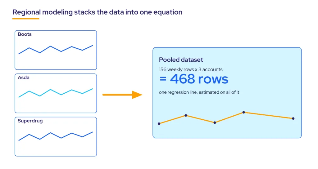
Take a product sold through three main UK retailers: Boots, Asda, and Superdrug. Suppose each has weekly data running from 1 January 2020 to 31 December 2022. That is three years, or roughly 156 weekly observations per account. Pool the three together and the dataset becomes 156 x 3 = 468 rows.
The number of observations roughly tripled. Ordinary least squares stacks the data from every account and fits a single regression line through all of it. That expansion buys three things: more robust measures, the ability to measure impact at the regional level, and the ability to capture more media granularity than a national model would support.
Three accounts of about 156 weekly observations each become one 468-row dataset, and every coefficient is estimated on all of it.
Pooling regions with different averages breaks OLS
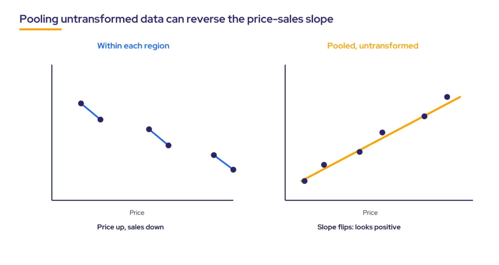
Pooled OLS behaves well only when the stacked regions sit at comparable levels. In practice they often do not. An analyst frequently pools high-selling regions with low-selling ones. Skip the transformation and run OLS on the raw data, and the model splits the difference: it overestimates sales in the regions that sell below the pooled average and underestimates them in the regions that sell above it.
The clearest example is price against sales. Look at each region on its own and the relationship is the expected one: when price rises, sales fall, and when price drops, sales rise. Pool several regions without transforming the data, fit one line through all the points, and the slope can flip. Price and sales appear to move together, which is the opposite of what economics and every individual region tell you.
Pool regions with different sales levels, skip the transformation, and OLS can quietly reverse the sign of your price coefficient. The model looks fine and the conclusion is wrong.
Normalization makes pooled regression valid
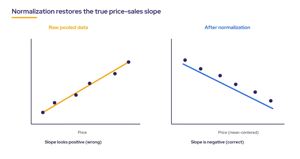
If the point of pooling is to read regional detail, you usually need to normalize the data first. There are several ways to do it: subtract the variable’s mean, divide it by its own mean, or divide it by the mean of the dependent variable.
Subtracting each region’s mean is worth naming precisely: it is the within transformation, which is exactly a fixed-effects specification. That is why analysts often call the pooled model, once normalized this way, pooled regression with fixed effects. Two cases need no separate step. Log-linear modeling normalizes through the log transform itself, so the data is already on a comparable scale. National models do not need normalization at all, because there is only one region. Normalized this way, the working assumption is that a variable’s effect is the same across regions in percentage terms, which is a fair default. We cover the log-linear route, and when to prefer it, in log-linear modeling for Marketing Mix Modeling.
Splitting variables captures different regional sensitivities
In MassTer, the Normalization processor handles this transformation, and estimating the pooled data then reports the average impact of each activity across all fitted regions. For a national TV campaign, that is the right default: you assume the percentage impact is equal across regions, and once you multiply it by the size of each region, the absolute impact is larger in bigger regions, which is what you would expect.
Sometimes that assumption is too strong. Some regions really are more sensitive to an activity than others. When an analyst models north against south and believes southern customers are more price-sensitive, the Splitter transformation lets them split the price variable across the two regions and estimate a separate coefficient, and therefore a separate elasticity, for each. The rule of thumb is simple: assume the same percentage contribution across regions by default, and split a variable only when there is reason to believe a region behaves differently.
We cover the mechanics of preparing and dividing those regional inputs in data splitting in Marketing Mix Modeling.
Partial pooling extends the same logic for 2026
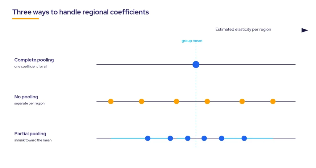
The choice between one shared coefficient and a separate coefficient per region is not binary. It is a spectrum, and pooled OLS and the Splitter sit at its two ends.
- Complete pooling (pooled OLS): one coefficient for every region. Efficient and stable, but it assumes regions behave identically in percentage terms once normalized.
- No pooling (per region): a separate coefficient for each region, which is the Splitter taken to its limit. Flexible, but small or sparse regions have too little data and their estimates get noisy.
- Partial pooling (hierarchical models): the model draws each region’s coefficient from a shared distribution, so every region’s estimate borrows strength from the others: it pulls small regions toward the group average while large regions keep their own signal.
Partial pooling is the idea behind geo-level Bayesian hierarchical MMM, the approach used in Google’s open-source Meridian and set out in Google’s research on geo-level Bayesian hierarchical media mix modeling. Meridian supports models with 50 or more geographies on two to three years of weekly data, and it produces tighter credible intervals for smaller markets precisely because it shares information across regions. Meta’s Robyn reaches for a different tool, regularized ridge regression, rather than a Bayesian hierarchy, but the goal is the same: stable, granular estimates when regions differ.
None of this replaces the pooled regression described above. It is the same instinct expressed with more statistical machinery. Complete pooling and no pooling are the extremes; partial pooling is the considered middle. Regression remains the engine, a point we make at length in why modern MMM still runs on its oldest engine.
| Approach | Complete pooling (pooled OLS) | No pooling (per region) | Partial pooling (hierarchical Bayesian) |
|---|---|---|---|
| Coefficients | One shared set across all regions | Independent set per region | Region-level, shrunk toward a shared mean |
| Small or sparse regions | Averaged into the pool, no local read | Noisy and prone to overfitting | Borrow strength from similar regions |
| Main risk | Masks genuine regional differences | High variance, unstable estimates | More complex to build and explain |
| Data appetite | Lowest | Highest | Moderate, handles uneven regions |
| MassTer lever | Normalization processor | Splitter transformation | Hierarchical / Bayesian layer |
| Verdict. Start with pooled OLS and normalization for most regional models. Split variables when specific regions clearly diverge. Move to partial pooling when you have many regions of uneven size and need stable, granular estimates for all of them. | |||
Frequently asked questions
Pooled regression, sometimes called panel regression, models data that has both a cross-sectional dimension (differences between regions, stores, or retailers) and a time-series dimension (change over time). In MMM it stacks several regions into one dataset and estimates a single equation, which lets you measure marketing impact below the national level.
Use it whenever the decision depends on regional detail: comparing stores, retailers, or markets, or measuring activity that only runs in some regions. A national model answers what moved total sales. A pooled model answers which regions moved and by how much, and it does so on a larger dataset, which makes every estimate steadier.
Pooled OLS assumes the stacked regions sit at comparable levels. When high-selling and low-selling regions are pooled without transformation, the model overestimates the low regions and underestimates the high ones, and it can even reverse the sign of a relationship such as price and sales. Normalization puts the regions on a comparable scale so the estimates stay honest.
No. Log-linear modeling normalizes the data through the log transform itself, so a separate normalization step is unnecessary. National models also do not need it, because they contain only one region. Normalization matters specifically for pooled linear models built across regions of different sizes.
Pooled OLS estimates one shared coefficient across all regions (complete pooling). A separate model per region estimates independent coefficients (no pooling). Hierarchical Bayesian MMM does partial pooling: each region gets its own coefficient, but those coefficients are drawn from a shared distribution, so small regions borrow strength from larger ones and estimates stay stable.
There is no fixed minimum, but more regions and more periods both help. As a reference point, geo-level Bayesian hierarchical models such as Google’s Meridian are built for 50 or more geographies on two to three years of weekly data. Pooled OLS works with far fewer regions, which is why it remains the practical default for most regional MMM projects.
For a fuller picture of what to gather before modeling, see the data required in Marketing Mix Modeling.
Conclusion
Pooled regression lets Marketing Mix Modeling measure below the national line, by store, retailer, product, or market. Pooling enlarges the dataset, which makes every measure more robust and makes regional effects visible in the first place. You estimate pooled OLS with ordinary least squares, and its validity depends on the stacked regions sitting on a comparable scale. When they are not, normalization keeps the results valid, unless you are already working in log-linear form, where the transform does the job for you.
For the fundamentals this builds on, from data preparation to model estimation, see our Comprehensive MMM Guide.
Those regional coefficients do not stay in the model either. They feed budget decisions downstream through response curves and channel synergy.
The deeper decision is how much to let regions differ. Assume one shared effect, allow every region its own, or let them share strength through partial pooling. Before your next regional model goes to a planning meeting, it is worth asking one question: are you assuming your regions behave the same because they do, or because you never checked?
- •Pooled regression models regions, stores, or retailers together in one equation, so you can measure marketing impact below the national level.
- •Pooling multiplies the dataset. Three retailers with about 156 weekly observations each become a single 468-row dataset, which steadies every coefficient.
- •Pooling regions of different sizes without normalization can reverse the sign of a coefficient, so normalize unless you are using log-linear modeling.
- •Subtracting each region’s mean is a fixed-effects specification; splitting a variable across regions estimates a separate elasticity where regions genuinely differ.
- •Partial pooling, the basis of hierarchical Bayesian MMM, is the middle ground between one shared coefficient and one per region, and it does not replace regression, it extends it.